This project was created using Power BI. In this project, I used various tools such as Dashboards – Data visualization, KPI, Extract, Transform, and Load (ETL), Graphs, Measures, Data modeling, Data cleaning.
Title:
Sales orders
Project Overview:
Summery:
Summery:
To do this project, I used the Northwind database, which contains sales data for many years of the fictional enterprise “Northwind Traders,”. I extracted the data from the kaggle site. In fact, this fictional enterprise is involved in global food import and export. The existing database has several files in CSV format and includes elements such as customers, orders, inventory, purchases, suppliers, shippers, employees. By using the data of this fictional enterprise, I reached achievements that can be useful for any real company to get an overview of the state of their company. Obviously, larger or smaller companies are always involved in ordering, buying, selling, and shipping similar to this company. All reputable companies need proper planning to calculate the following:
Receiving product orders, timely delivery to the customer, estimation of the amount and average sales, delay in the shipment and the percentage of shipment not shipped.
Using Power BI software allows us to use data modeling and data visualization to analyze the company’s situation at any moment and predict a picture of the future.
Database:
Database contains the entities below:
There are 6 CSV files whose fields and records are as follows:
Customers: Customers who buy products from Northwin:
9 fields & 91 records
Companyname, Contactname, Contacttitle, City, Region, Postalcode, Country, Phone, Fax.
Orders: Sales Order transactions taking place between the customers & the company:
14 fields & 830 records
Orderid, Customerid, Employeeid, Orderdate, Requireddate, Shippeddate, Shipvia, Freight, Shipname, Shipcity, Shipregion, Shippostalcode, Shipcountry, Shipperid
Order_Details: Sales Order transactions taking place between the customers & the company
5 fields & 2155 records
Ordered, Productid, Unitprice, Quantity, Discount.
Products: Product information
10 fields & 77 records
Productid, Productname, Supplierid, Categoryid, Quantityperunit, Unitprice, Unitsinstock, Unitsonorder, Reorderlevel, Discontinued.
Shippers: The details of the shippers who ship the products from the traders to the end-customers:
3 fields & 7 records
Shipperid, Companyname, Phone
Suppliers: Suppliers information and vendors of Northwind:
12 fields & 29 records
Supplierid, Companyname, Contactname, Contacttitle, Address, City, Region, Postalcode, Country, Phone, Fax, Homepage.
Questions & Goals:
- Data cleaning
- Data modeling
- What is the maximum amount of sales for different orderids?
- What is the percentage of sales orders that have not been shipped?
- What is the average sales amount?
- How much is the total of freight? How much is the freight per order?
- How many days has the company delayed in shipping orders?
- What are the top 5 products by destination country?
- How can the quantity of sold products be checked dynamically along with the changes of other items?
- What is the total amount of sales based on the company name?
- What is the total amount of discounts for each supplier?
- How has the total freight rate changed from 1996 to 1998?
- What is the total freight based on the shipcountry?
Steps:
I designed a sales analysis dashboard using the data of an fictional enterprise, and by using DAX expressions in Power BI software, I was able to merge several tables in CSV format in Excel. And finally, I designed a new model of the company’s sales and shipping orders and presented the company’s dynamic analytical dashboard with data visualization. In the first step, I performed data cleaning using ETL in the power query section, and then I designed a model for the data in the View Model section.
Data Cleaning:
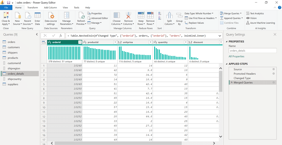
Customer id, Shipcountry, Shipregion: To create a relationship between the tables, I had to make the fields unique. So, in the power query section, I first duplicated the required fields and then made them unique.
Orders: In the next step, there were two orders tables that I merged.
Customers: The naming of the headers of this table was changed to “Column” in the loading process, which was modified using the CSV source file.
Shippeddate: This field contained the shipping dates of the goods, which were stored in the format of day, month, year, and hour. While the orderdate and requiredate fields were saved without recording the time. In order to unify the format of these, I used “Split”, “Remove duplicate” and “Duplicate column” tools.
Finally, I saved the changes and arranged the tables ready for model design.
Data Modeling:
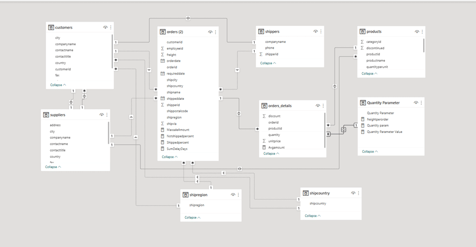
Power BI Data Model Analysis and Interpretation:
The data model designed in this Power BI project follows a Star Schema structure, aimed at providing a comprehensive analysis of sales performance, customers, products, suppliers, and shipping operations within the organization.
By integrating several key tables including Orders, Order_Details, Customers, Products, Suppliers, and Shippers the model enables a detailed examination of the relationships across various components of the sales process.
Structure and Relationships
In this model, the Order_Details table functions as the fact table, containing detailed transaction-level information such as unit price, quantity, and discount for each order.
The supporting dimension tables such as Customers, Products, Suppliers, and Shippers provide descriptive attributes that allow data analysis from multiple perspectives, including customer demographics, product categories, supplier performance, and shipping logistics.
One-to-many (1:*) relationships between these tables are properly defined, ensuring accurate data filtering, aggregation, and cross-table analysis throughout the model.
Key Analytical Insights
Using this model, the following analyses can be performed:
1-Sales and Revenue Analysis:
Calculation of total and average sales, identification of top-selling products and customers, and evaluation of sales trends over time.
These insights help decision-makers focus on the most profitable market segments.
2-Customer Analysis:
Examination of customer distribution by region, total purchase volume per customer, and identification of loyal or high-value customers.
3-Supplier Analysis:
Evaluation of supplier performance based on product sales volume, product variety, and contribution to overall sales.
4-Shipping and Logistics Analysis:
Comparison of shipping companies’ performance based on the number of orders delivered, shipping times, and delay percentages.
5-Geographical Analysis (Region & Country):
Integration of ShipCountry and ShipRegion tables allows spatial analysis of sales performance and helps identify potential markets for expansion.
6-Dynamic Parameterized Analysis:
The Quantity Parameter table introduces interactive analysis, enabling users to dynamically switch between analytical metrics such as quantity, freight cost, or order volume.
Conclusion
The developed data model provides a cohesive, scalable, and analytically rich foundation for business intelligence reporting. It delivers not only a holistic overview of sales and operational performance but also supports advanced multidimensional analysis empowering strategic decisions in areas such as marketing, supply chain, and logistics management. By incorporating additional measures such as Gross Profit, Delivery Delay Rate, and Product Market Share, the model can serve as the analytical core of an intelligent decision-support system for the organization.
The way to connect the dimensions is as follows:
Company name (Shippers, Customers)
Customer id (Orders , Customers)
Phone (Customers, Supplier )
Shipper id (Orders, Shippers)
Country (Customers, Ship country)
Order id (Orders, Order-details)
Region ( Customers, Ship region)
Ship country( Orders, Ship country)
City( Customers , Orders , Suppliers)
Product id (Product, Order-details)
Ship region ( Orders, Ship region)
Supplier id( Product, Supplier)
Quantity (Order-detail , Quantity parameter)
Analysis:
After preparing the data and data modeling, in order to reach the answers to the desired questions and goals, I have to write the required measures using DAX.
-Maximum amount of sales for different orderids
In order to get the maximum sales amount, I first chose the name of the “sales amount” and calculated it based on the “quantity” and “unit price”. Then I created a measure:
MaxSaleAmount = Maxx(SUMMARIZE(‘order (2)’, ‘order (2)’[ordered], “salesAmount”, SUMX,(order_details, order_details[quantity]* order_details[unitprice])),[saleAmount])
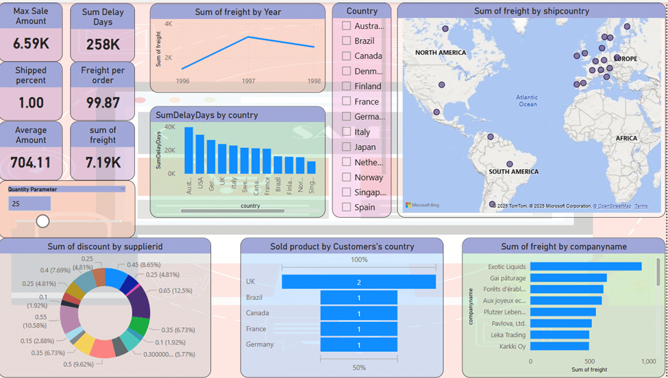
The given KPI illustrates the maximum sales amount for different orderids in destination countries between 1996 and 1998. It is evident that the highest sales amount based on quantity of items and unit price was $6.59 thousand.
-The percentage of sales orders that have not been shipped
To get the percentage of undelivered commodity, I created a measure based on total freight and shipping date. Based on this, the percentage of commodity delivered was obtained by subtracting the number 1 from the percentage of commodity undelivered, which was calculated in another measure:
Notshippedpercent = CALCULATE(SUM(‘order (2)’[freight]), ISBLANK(‘order (2)’[shippeddate])=TRUE())/SUM(‘order (2)’[freight])
Shippedpercent = 1- Notshippedpercent
The KPI illustrates that all orders have been shipped and the company has experienced 100% sales of its products. Overall it is apparent that there was maximum sales from 1996 to 1998. Moreover, the percentage of products not shipped is zero.
-Average sales amount
To calculate the average sales, I used the name “Avgamount” and created a measure based on the quantity and unit price:
Avgamount = AVREGEX (order_details, order_details [quantity] * order_details [unitprice])
The KPI depicts the average amount sales in the hypothetical company. In general, it is evident that average sales was approximately $ 704,000 from 1996 to 1998.
-How much is the total of freight? How much is the freight per order?
One of the cost items in a company’s budget is freight. In this section, we want to examine how much the total freight is and how much the average freight cost is for each item.
The given KPI illustrates the total freight was approximately $7000 between 1996 and 1998. To get the freight per order, I created a measure:
freightperorder = SUM(‘orders (2)’ [freight])/COUNT (‘orders (2)’[orderid])
Overall, freight per order was generally approximately $ 100. Looking at the average sales in more detais, the total freight saw nearly to one hundredth of the average sales, which was low cost shown on the costs of sales.
–How many days has the company delayed in shipping orders?
I created another measure called “SumDelayDay”, which calculates the number of days that the goods were sent late. This item was created based on “requireddate” and “shippeddate” fields:
SumDelayDays = CALCULATE(SUMX(‘orders’(2), DATEDIFF(‘orders(2)’[requireddate], ‘orders(2)’[shippeddate],DAY)), DATEDIFF(‘orders(2)’[requireddate], ‘orders(2)’[shippeddate],DAY)>0)
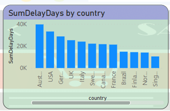
The KPI shows that the total number of daily delays in shipping goods to different countries. In general, it evident that the sum of delay days was 258,000 days between 1996 and 1998.
Given is a bar graph prviding comprehensive information on the numbers of delay days in shipping the goods comparison of various countries. Looking from an overall perspective, it is starkly apparent that, Australia and after that USA had the most delay days in receiving the goods, while Denmark had the less delay days around 3360, which you scroll and see it. In terms of Australia and USA, while the number of delay days in shipping the goods of USA was about 33153, the figure for Australia was slightly higher, at around 39581. Meanwhile, over 70,000 of 258,000 delay days were relaited Australia and USA. As a result at approximately One-third of the number of days is related to these two countries. Whereas the number of delay days in shipping goods to other countries is 188,000 days. Moving on to the remaining countries, having the lowest delays in shipping after Singapore were Norway, Finland, and Brazil at approximately 15,000 that a close similarity can be seen in that countries. At the same time, over 20,000 days for France, Canada, Sweden,compared to over 25,000 days Italy, England and Germany respectively. Finally, the number of days of delay can be high or low depending on the distance to the destination country, the type of shipping, the shipping cost, and the strength or weakness of the service.
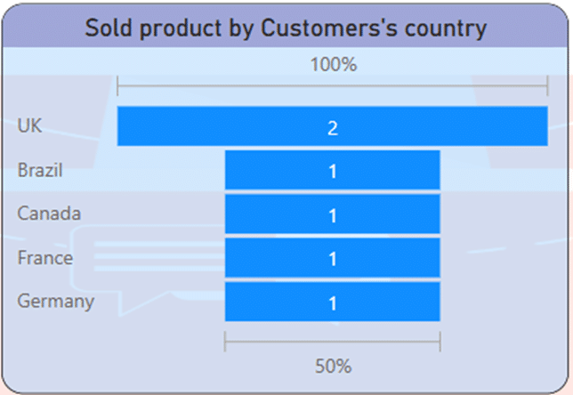
The top 5 products by destination country
I created a measure to display the top 5 products that had the most sales in the countries. I finally displayed it in a bar chart:
TOP 5 pr by co = VAR TOPPRODUCTS = TOPN(5, ADDCOLUMNS(VALUES(‘product’[productname]),
”salesAmount”, [Total sales]),
[salesAmount],
DESC)
RETURN
IF(
CONTAINS(TOPPRODUCTS, products[productname],SELECTEDVALUE(‘product’[productname])), [Total sales],
BLANK()
)
This bar chart illustrates the top five selling products across different countries. Each color represents a distinct product, while the height of each bar indicates the total sales value within that country. The main purpose of this visualization is to compare product performance across international markets and identify key areas of strength.
Key Observations:
France:
France shows the highest total sales, reaching around 6,000 units. The top-performing product is Côte de Blaye, which significantly outperforms other products in all countries. This suggests a strong consumer preference and market potential for this product in France.
Germany:
Ranked second in total sales (approximately 2,000 units). The leading product is Chang, indicating solid market demand within Germany. The sales gap between Germany and France is notable, implying differences in customer preferences or pricing strategies.
Canada:
Shows moderate sales performance (around 1,000–1,500 units). The most popular product is Pâté chinois, reflecting unique consumer tastes in the Canadian market.
Brazil:
Exhibits lower sales levels compared to other countries. The top-selling product is Guaraná Fantástica, which aligns with local beverage preferences in South America.
United Kingdom (UK):
Has the lowest sales volume among the analyzed countries.
The primary product sold is Schoggi Schokolade, suggesting a niche market with limited overall demand.
Comparative Insights:
France stands out as the most profitable and promising market, indicating high demand and sales concentration. Germany and Canada represent stable but moderate markets with room for growth through targeted promotions or expanded product lines. Brazil and the UK display weaker market performance, suggesting the need for revised pricing, marketing, or distribution strategies.
The analysis reveals clear geographical variations in product performance. Côte de Blaye dominates in France and should be prioritized in European market strategies. A segmented marketing approach is recommended, tailoring product focus and promotional efforts to each country’s consumer behavior. Overall, this visualization helps identify key growth opportunities and supports data-driven decision-making for international sales optimization.
-How can the quantity of sold products be checked dynamically along with the changes of other items?
I defined a parameter called Quantity parameter, which by changing it between 0 and 100 quantity of goods, changes in the average amount of sales are displayed. This parameter dynamically affects other charts. For this purpose, I created three measures:
The change of the parameter shows the quantity of sold goods, which can be used to see the changes of other charts.
Quantity parameter = GENERATESERIES(0, 100, 1)
Quantity parameter value = SELECTEDVALUE(‘Quantity parameter’ [Quantity parameter])
Quantity param = SUMX(FILTER(‘orders_details’, ‘orders_details’[quantity]<’Quantity parameter’[Quantity parameter value], ‘orders_details’[Avgamount])
–What is the total of freight based on the company name?
Since the company has agencies in different countries. You can check the freight based on the name of the dealers.
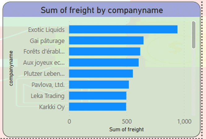
The bar chart compares the different companies in all of the world in terms of sum of the freight between 1996 and 1998. Overall, the freight was generally the most amount in “Exotic liquids” company, while the freight was the least in “Tokyo Traders” company apprpximately 27, which you scroll and see it. Looking at seven companies except for “Exotic liquids” company which was nearly 1000 in the freight amount, “Gai patorage” company saw that the freight was 649, which was the largest amount shown on the chart after “Exotic liquids” company, compared to “Forets d erables” and “Aux Joyeux ecclesiastiques” over 600 slightly. These figures all were the largest freight amount in these companies. In fact, between the most and the least freight amount in these companies , more specifically, there was over 900 difference that was around 35 times. This discrepancy is strikingly high and its reasons should be investigated with more information.
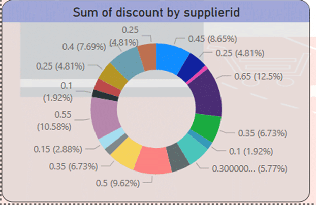
-What is the total amount of discounts for each supplier?
The donut chart illustrates the distribution of total discounts offered by each supplier. The results indicate that discount allocation is highly concentrated among a few key suppliers. Supplier 0.65 accounts for the highest portion of discounts with 12.5%, followed by suppliers 0.55 (10.6%) and 0.50 (9.6%). Together, these three suppliers represent approximately one-third of the total discount volume. This suggests that they either handle a larger share of sales or adopt more aggressive pricing strategies to maintain competitiveness.
In contrast, the remaining suppliers contribute smaller shares ranging between 4% and 8%, showing a relatively diversified but unequal distribution. Overall, the pattern highlights that a limited number of suppliers play a dominant role in discounting activities. The focus of discounts is on a few specific suppliers.
The three main suppliers (0.65, 0.55 and 0.5) together account for about 32% of all discounts.
This means that discount policies are more focused on products in this group. These suppliers probably have a higher share of sales or are more price competitive and offer higher discounts to attract customers. The distribution of discounts is relatively diverse, but uneven. That is, not all suppliers have an approximately equal share, and a few major suppliers determine the overall discount pattern. If this data is compared to Sales Amount, it can be examined whether high discounts have also led to increased sales a useful analysis for future marketing and purchasing decisions.
It is recommended to further compare discount values with total sales amounts to evaluate whether higher discounts have effectively driven increased sales performance or simply reduced profit margins.
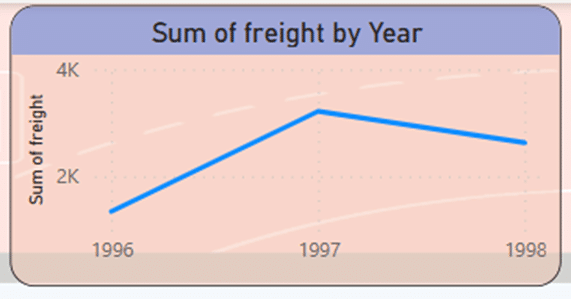
How has the total freight rate changed from 1996 to 1998?
Using a line chart, the company’s total freight are displayed in the period of 1998-1996. As the diagram shows; total freight grow from 1996 to 1997 and reach their highest level in 1997. After that, there is a downward slope, which should be investigated, what was the reason for the decrease in freight in 1998.
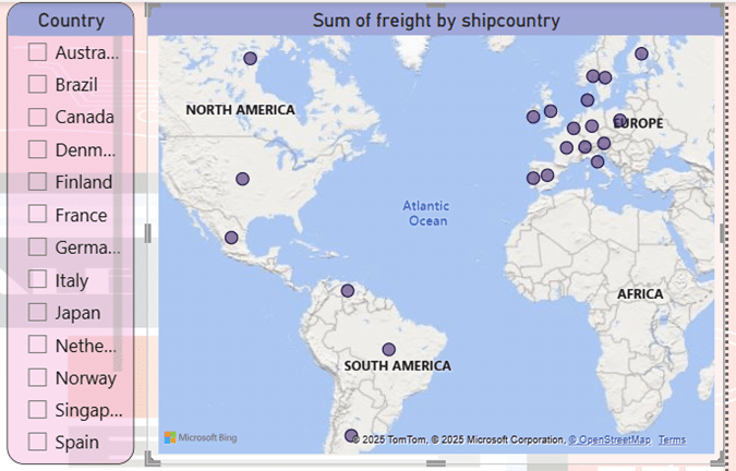
-What is the total freight based on the shipcountry?
This map visual displays the total freight cost distributed across different shipping destination countries. Each circle on the map represents a country, and the size of the circle corresponds to the total amount of freight associated with that country. The visualization shows that European countries (such as France, Germany, Italy, Spain, and the Netherlands) have the highest freight sums, indicating that a large portion of shipping activity is concentrated in Europe. This suggests strong trading relationships and high shipment volumes within this region.
In contrast, North American countries such as the United States and Canada show moderate freight totals, while countries in South America (e.g., Brazil) and Asia-Pacific (such as Japan, Singapore, and Australia) display relatively smaller freight sums. These regions may represent either smaller market shares or less frequent shipments compared to Europe. From a business perspective, the map highlights that Europe is the dominant freight destination, which could imply that the company’s logistics network and customer base are primarily centered in that region. This information is valuable for optimizing shipping routes, negotiating logistics costs, and identifying potential opportunities for market expansion in underrepresented regions.
Key points:
- The data model designed in this Power BI project follows a Star Schema structure, aimed at providing a comprehensive analysis of sales performance, customers, products, suppliers, and shipping operations within the organization.
- The highest sales amount based on quantity of items and unit price was $6.59 thousand between 1996 and 1998.
- The company has experienced 100% sales of its products. Overall it is apparent that there was maximum sales from 1996 to 1998. Moreover, the percentage of products not shipped is zero.
- Average sales was approximately $ 704,000 from 1996 to 1998.
- The total freight was approximately $7000 between 1996 and 1998.
- Freight per order was generally approximately $ 100.
- The total freight saw nearly to one hundredth of the average sales, which was low cost shown on the costs of sales.
- The sum of delay days was 258,000 days between 1996 and 1998.
- Australia and after that USA had the most delay days in receiving the goods, while Denmark had the less delay days around 3360.
- In terms of Australia and USA, while the number of delay days in shipping the goods of USA was about 33153, the figure for Australia was slightly higher, at around 39581. Meanwhile, over 70,000 of 258,000 delay days were relaited Australia and USA. As a result at approximately One-third of the number of days is related to these two countries.
- France shows the highest total sales, reaching around 6,000 units. The top-performing product is Côte de Blaye, which significantly outperforms other products in all countries. This suggests a strong consumer preference and market potential for this product in France.
- Germany ranked second in total sales (approximately 2,000 units). The leading product is Chang, indicating solid market demand within Germany. The sales gap between Germany and France is notable, implying differences in customer preferences or pricing strategies.
- Canada shows moderate sales performance (around 1,000–1,500 units). The most popular product is Pâté chinois, reflecting unique consumer tastes in the Canadian market.
- Brazil exhibits lower sales levels compared to other countries. The top-selling product is Guaraná Fantástica, which aligns with local beverage preferences in South America.
- United Kingdom (UK) has the lowest sales volume among the analyzed countries.
- The primary product sold is Schoggi Schokolade, suggesting a niche market with limited overall demand.
- The freight was generally the most amount in “Exotic liquids” company, which was nearly 1000 in the freight amount, while the freight was the least in “Tokyo Traders” company apprpximately 27.
- The remaining suppliers contribute smaller shares ranging between 4% and 8%, showing a relatively diversified but unequal distribution.
- The three main suppliers (0.65, 0.55 and 0.5) together account for about 32% of all discounts.
- Total freight grow from 1996 to 1997 and reach their highest level in 1997. After that, there is a downward slope, which should be investigated, what was the reason for the decrease in freight in 1998.
- North American countries such as the United States and Canada show moderate freight totals, while countries in South America (e.g., Brazil) and Asia-Pacific (such as Japan, Singapore, and Australia) display relatively smaller freight sums.
- From a business perspective, the map highlights that Europe is the dominant freight destination, which could imply that the company’s logistics network and customer base are primarily centered in that region.
Results & Recommendations:
- The state of the company from 1996 to 1997 has economic growth and prosperity. The slope of sales is upward, but between 1997 and 1998, the slope suddenly becomes downward. The reasons for that should be investigated. It is suggested to focus on customer satisfaction, product quality, price, and delivery method.
- The amount of production and sales seems to be excellent. But the trend of sales growth is negative. The amount of sales should be checked over time.
- Regarding the delay in sending products to different countries, especially Australia, it should be reconsidered. Means of transportation, equipment for receiving and sending orders, the number of workers must be managed.
- It seems that the biggest weakness of the company is the delay in sending the goods, which should be seriously addressed, maybe this is the reason for the downward slope in sales.
- The amount of sales in Europe is good, but it seems low in other places. Advertising of goods and products should be planned and promoted according to the needs of each country.
- The percentage of discounts is low. It should be agreed with the suppliers during meetings to consider more discounts, for this purpose holding events can be effective.
- It is necessary to increase the functionality and production of differentiated products.
- It is recommended to further compare discount values with total sales amounts to evaluate whether higher discounts have effectively driven increased sales performance or simply reduced profit margins.
- Companies with high performance should be encouraged and their performance should be set as a model.
Action
In this project, In this project, I used simple functions, clauses and query options to get my answers:
Aggregate Functions: SUM, COUNT, SUMX, MAXX,
Functions Clauses: SUMMARIZE, CALCUATE, ISBLANK, TRUE, DATEDIFF, DAY, AVERAGEX, DISTINCTCOUNT, FILTER, SELECTEDVALUE, GENERATEDSERIES, ADDCOLUMNS, DESC, RETURN, IF, CONTAINS, BLANK. Query Options: DIPLICATE COLUMN, CHANGE TYPE, MERGE QUERIES, RENAME COLUMN,REMOVE DUPLICATE, SPLITE.
Link:
Thank you so much for reading my project. I will be happy to receive your feedback and opinion about the project. If this project is useful for you, click on this link:
Link to project repository on GitHub
Link to project video on LinkedIn
Link of CSV Northwind Database on Kaggle