This project was created and analyzed using Excel ,Power Bi, SPSS & Word. In this project, I used various tools such as:
Excel Using: Dashboard, Pivot table, Conditional formatting and Formulas, Data visualization
Power Bi: Dashboard, Graphs, KPI, Measures, Data visualization
SPSS Using: Frequency Distribution, Converting a quantitative variable into a categorical variable, Tests related to comparing the frequency and mean of two independent groups, Outlier Data, K-means clustering, Graphs, Two-stage clustering of the likelihood function, Non-parametric tests
Word: Text typing, page layout and table drawing
Title:
An analysis of the proposed plan to standardize IRIB pensions:
Project Overview:
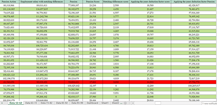
Database, 2020
Summery:
The project of standardize IRIB pensions is one of the important projects in progress in the IRIB organization. This project has a massive data and complex calculation formulas. When I was working with the organization, I used to participate in the review meetings of the proposed plans. After I retired, I decided to analyze one proposal that I thought was stronger than the others. This project had a massive data including the information of more than 16 thousand retired people of the organization, which required a lot of time and accuracy to review and analyze. Due to the vastness of the content, I finally decided to publish it as a book and make it available to the stakeholders. Standardize IRIB pensions is not only for the IRIB organization, but also it is a government concern. The goal is to try to reduce the gap between low and high levels of pensions and create a balance between the pensions and expenses of retirees according to the inflation in the society. The start of this work was from January 2023, but I did not work on the project continuously due to personal problems. And since the said project had many details and the collection of documents took a lot of time, finally in January 2025, the project was published in the form of a book. Because the contents of the book are very extensive and it is not possible to include all the contents here, I translated some parts of the book and put them on my website.
Database:
The basic data of this project was extracted from the information of IRIB retirees from 1973 to 2020, whose table was designed on Excel. This table had 16,744 rows and 126 columns. After cleaning the data and removing the columns that did not affect the analysis and the columns that were hidden, I added three more columns to the table, which were: “Percentage of salary increase, outlier data and amount of salary increase” and finally I edited the new table with 117 columns. Due to the large volume of the data file, it was not possible to include all its pages in this collection. Therefore, in order to display the database as a whole, the first 22 rows were randomly selected and the images of all its columns were placed except for the employee number and first and last name columns. These images can be seen in the attachments section. The columns of the edited table of information are:
A: ID AA: Work place
B: Name AB: Department of work place
F: Start date AC: Deprivation of facilities
H: Retirement date AD: Boundary amount
I: Degree score AE: Transfer amount
J: Job coefficient AF: Transfer by the organization’s request
K: Job score AG: Bad weather amount
L: Individual score AH: Deprived areas amount
M: Absorption coefficient AI: Percentage of deprived areas
N: Equivalent degree AJ: Hard work
O: New degree score AK: Hard work of mast repairman
P: Job title AL: Special areas
Q: New job score AM: Management level score
R: Coefficient of new job AN: Management coefficient
S: Coefficient of selection administration AO: Level management
T: Human resources coefficient AP: Management reward score
U: Protection coefficient AQ: Veterans score
V: Violation coefficient AR: Veterans salary
W: Engineering AS: Salary without veterans score
X: Legal coefficient
Y: Experiences by month
Z: New individual score = Individual score * 4.4
AT: Basic salary = (New individual score + New job score + New degree score) * 1.43 * 3353
AU: Job additional amount = (New job score + New degree score) * (Violation coefficient + Protection coefficient + Human resources coefficient + Coefficient of selection administration + Job coefficient) / 100 + 6530 * 1.43 * 3353
AV: Management amount = (New degree score + New job score) * (Management coefficient / 100) * 1.43 * 3353
AW: Management experiences
AX: Veterans amount
AY: The amount of Article 51
AZ: Matching difference score amount
BA: The sum of the salary personal action that can be calculated for retirement = Job additional amount + Basic salary + The amount of Article 51+ Veterans amount + Management amount + Management experiences
BB: The sum of the final salary of the time of employment with the matching difference score amount = Matching difference score amount + The sum of the salary that can be calculated for retirement
BC: Pension = The sum of the salary that can be calculated for retirement * 97%
BD: Pension score = Pension / 3353
BE: Matching difference score = Matching difference amount / 3353
BF: Retirement scores by applying the years deduction work experiences = Retirement scores * Experiences by month / 300
BG: Pension with the application of the years deduction of work experiences = Retirement score with deduction of years of work experiences * 3353
BH: The final standardize retirement score = Retirement score with deduction of years of work experiences + Matching difference score
BI: Standardize final pension = Standardize final pension score * 3353
BJ: Score difference = Standardize final pension score – veterans score
BK: Rials difference = Score difference * 3353
BL: Percentage increase = Score difference / Score with veterans * 100
BM: The amount engineering = (Degree score + New job score) * 38% * 1.43 * 3353
BN: The technical amount = 350,000 Rials or 400,000 Rials (It is determined based on the job title.)
BO: Legal expert amount = (New degree score + New job score) * Legal expert amount coefficient / 100 * 1.43 * 3353
BP: The amount medical (Specialist doctor) = 2800 * 3353 * 1.43
The amount medical (General Practitioner) = 2200 * 1.43 * 3353
BQ: The amount radiation (Specialist doctor) = 2800 * 1.43 * 3353
The amount radiation (General practitioner) = 2200 * 1.43 * 3353
BR: The sum of job additional amount = The amount radiation + The amount medical + The amount Legal expert + The amount Technical + The amount Engineering
BS: The sum of amount pensions related to job = The sum of job additional amount * 97%
BT: The sum of job additional amount scores = The sum of amount pensions related to job / 3353
BU: The sum of job additional amount scores with deduction of years of work experiences = The sum of job additional amount score * Experiences by month / 300
BV: The sum of job additional amount salary with deduction of years of work experiences = The sum of job additional amount scores with deduction of years of work experiences * 3353
BW: The amount of deprivation of facilities = (38% * basic salary) *Coefficient of deprivation of facilities / 100
BX: The amount border = (38% * Basic salary) * Border coefficient / 100
BY: The amount transfer = (38% * Basic salary) * Transfer coefficient / 100
BZ: The amount bad weather = (38% * Basic salary) * Bad weather coefficient / 100
CA: The amount deprived areas = (New degree scores + New job scores) * 32% * 1.43 * 3353 * Coefficient of deprived areas / 100
CB: The amount hard work = (38% * Basic salary) * (Hard work of mast repairman * Hard work coefficient) / 100
CC: The sum of additional amount of work place = The amount hard work + The amount deprived areas + The amount bad weather + The amount transfer + The amount border + The amount deprivation of facilities
CD: Pension Action= Sum of final salary during employment with matching difference score + The sum of job additional amount salary with deduction of years of work experiences + The sum of additional amount of work place.
CE: The sum of additional amount of retirement work place = The sum of additional amount of work place * 97%
CF: The scores additional amount of work place = The sum of additional amount of retirement work place / 3353
CG: The sum of the scores additional amount of work place with deduction of years of work experiences = the scores additional amount of work place * experiences by month / 300
CH: The sum of salary additional amount of work place with deduction of years of work experiences = The sum of scores additional amount of work place with deduction of years of work experiences * 3353
CI: Overtime = (The sum of the salary that can be calculated for retirement / 160) / 2.2 * overtime hours
(Explanation: overtime limit of 150 hours)
CJ: Overtime hours = 150 hours
CK: Shift work = (38% * Basic salary) * Shift work coefficient / 100 * Number of shifts
(Explanation: 12 Shift work shift limit)
CL: Coefficient of shift work
CM: Number of shifts
CN: Management reward = (Management reward score * 1.43 * 3353)
CO: Sum of perks = Overtime + Management reward
CP: Sum of retirement perks = Sum of perks * 97%
CQ: Retirement perks score = Sum of retirement perks / 3353
CR: Perks score with deduction of work experiences = Retirement benefits score * Experiences by month / 300
CS: Perks salary with deduction of work experiences = Perks score with deduction of work experiences * 3353
CT: Sum of pension scores = Standardize final pension scores + The sum of scores job additional amount with deduction of years of work experiences + The sum of scores work place additional with deduction of years of work experiences + Perks score with deduction of work experiences
CU: Sum of pensions = Sum of pensions scores * 3353
CV: Difference of scores with perks = Sum of retirement scores – Scores with veterans
CW: Rials difference with benefits = Scores difference * 3353
CX: Percentage increase in perks with previous salary = Scores difference / Scores with veterans * 100
CY: Increase in perks with standardize salary = (Final scores of standardize pension – Sum of pension scores) / Final scores of standardize pension * 100
CZ: Sum of salary bills = Sum of pension action + Sum of perks
DA: Monthly perks at the time of employment = The sum of amount job scores + The sum of additional amount of work place + Sum of perks
DB: Scores of monthly perks at the time of employment = monthly perks at the time of employment/ 3353
DC: Monthly perks at the time of employment 1400 = Scores of monthly perks at the time of employment * 3048
DD: Monthly perks at the time of employment in 1399 = Scores of monthly perks at the time of employment * 2438
DE: Monthly perks at the time of employment in 1398 = Scores of monthly perks at the time of employment * 2120
DF: Monthly perks at the time of employment in 1397 = Scores of monthly perks at the time of employment * 1797
DG: The contribution of the organization with 24 months = ((12 * Monthly perks at the time of employment) + (12 * Monthly perks at the time of employment 1400)) * 16%
DH: Employee contribution with 24 months = ((12 * Monthly perks at the time of employment) + (12 * Monthly perks at the time of employment 1400)) * 8%
DI: Total sum of 24 months = Employee share with 24 months + Organization share with 24 months
DJ: 24 monthly installments = employee contribution / 24
DK: The contribution of the organization with 60 months = {(12 * monthly perks at the time of employment) + (12 * monthly perks at the time of employment in 1400) + (12 * monthly perks at the time of employment in 1399) + (12 * monthly perks at the time of employment in 1398) + (12 * monthly perks at the time of employment in 1397)} * 16%
DL: Employee contribution for 60 months = {(12 * monthly perks at the time of employment) + (12 * monthly perks at the time of employment in 1400) + (12 * monthly perks at the time of employment in 1399) + (12 * monthly perks at the time of employment in 1398) + (12 * monthly perks at the time of employment in 1397)} * 8%
DM: Total sum 60 = employee share 60 + organization share 60
DN: 60 installments = employee share 60 / 60
DO: Salary increases percentage = The sum of the salary that can be calculated for retirement – sum of pension / The sum of the salary that can be calculated for retirement * 100
DP: Outlier data = Data whose salary increase percentage is less than 27% or more than 47%.
DQ: The amount of salary increase = The sum of the salary that can be calculated for retirement – the sum of pensions
Questions & Goals:
1-What is the amount and percentage of income increase for the lowest and highest salaries compared to the income before standardize?
2-Are the percentage distribution of salary increases normal after standardize?
3-Is the frequency distribution of all educational levels the same?
4-Do the levels of educational qualifications have a significant effect on the percentage of salary increase?
5-Is there a significant difference in the average amount of benefits in different groups?
6-What is the trend of changes in benefits compared to changes in standardize salary?
7-Is there a significant difference in the average percentage increase in standardize between different occupational groups?
8-Are the rankings of salary variables significantly different from each other?
9-What is the average benefits for different groups?
10–What is the average percentage of salary increase after standardize in different groups?
11-Difference in pension increase percentage according to job grouping
12-Is there a significant difference in adding the matching difference score in the final standardize retirement score?
13-Are the ranking of the independent salary variables different from each other significantly?
14-Clustering pensions by their increasing percentage.
15-If the model has outliers, how can they be identified and corrected?
16-Average salaries before and after standardize for non- veterans’ employees?
17-The effect of retirement date on the rate of increase in non- veterans’ employees.
18-Average effective points in the percentage of salary increases for non- veterans’ employees.
19-Comparison of the difference of matching score and benefit score
20-Comparison of pre-standardize salaries and increase amounts for non- veterans’ employees.
21-Comparison of the contribution of standardize points to the final retirement points for non- veterans’ employees
22-Details of changes before and after standardize for non- veterans’ employees.
23-Comparison of salaries before and after standardize of veterans’ managers in Tehran and Qazvin.
24-Comparison of the percentage of salary increases for veterans’ managers in Tehran and Qazvin.
25-Is the amount of salary increase and the share of installment payments suitable for veterans’ managers?
26-Comparison of average reward scores, experience, and management level, and veterans score in the salaries of veteran’s managers.
27-Comparison of salaries before and after standardize and the percentage increase in salaries of radio and television producers in Tehran and Hamadan for non-veterans employees.
28-Comparison of salaries before and after standardize and the percentage increase in salaries of technical engineerin Tehran and Zahedan for non-veterans employees.
29-Comparison of salaries before and after standardize and the percentage increase in salaries of system expert Tehran and Sanandaj for non-veterans employees.
30-Comparison of salaries before and after standardize and the percentage increase in salaries of news editor and reporter of Tehran and Yazd for non-veterans employees.
31-Comparison of salaries before and after standardize and the percentage increase in salaries of media protection employee of Tehran and Isfahan for non-veterans employees.
32-Details of changes before and after standardize for non- veterans’ employees.
Steps:
The project of standardize IRIB pensions:
In this proposed plan to standardize IRIB pensions, it is tried to solve the above problems by using the social security model and create a combination of the organizational model and the social security model. For this purpose, information related to retired points for job, educational qualification, veterans , place of work, management, etc., from 3/3/1974 to 6/21/2020 for the number of 16,746 retired, in a table and updated. Formulas and salaries changes were calculated and determined based on new points.
In the next step, the last pay slip of the employment status of the retired was checked and their salaries items that were not included in the pension were extracted. Among these following items were not included in the calculations due to the difficulty of receiving updated information at the time of project implementation. Obviously, in case of agreement with the implementation of the plan, the following will also be considered:
The salary of medical technical responsibility, amount exclusion from the office; The salary to be responsible for storage; The salary of the property trustee; The salary of knowledge and maintenance of equipment and goods.
Also, shift work that can be paid for the organization’s shift jobs, due to not receiving the updated list at the time of project implementation, was not included in the calculations; But the formula and how to calculate it is placed in the table, and instead, all employees are given 150 hours of overtime by default, which is not much different compared to people who receive shift work and do not receive overtime.
The amount special expertise/skill that was approved in 2018 and the amount special national media approved in 2022 are also not included in the salary calculations due to different implementation dates.
The general formula for calculating standardize pension is calculated as follows:
Sum of retirement points = {(Final standardize pension score) + (The sum of job additional amount scores with deduction of years of work experiences) + (The sum of additional amount of work place scores with deduction of years of work experiences) + (Perks score listed in the last pay slip with deduction of years of work experiences)}
Standardize pension = sum of pension points * Rials coefficient of the year of implementation of the plan
Description:
1-The final standardize pension score = {(The sum of the amount of continuous the last salary personal action that can be calculated for retirement) * (Rials coefficient of the year of implementation of the plan) * 97% * (Experiences by month / 300) + matching difference score}
2-25 years of full operation per month = 300 months
3-Matching difference score = matching difference amount / riyal coefficient of the plan implementation year
Note: If after the issuance of the last salary personal action, the amount of continuous pensions of the previous people was lower, this amount will be included as a difference of adjustment in the new personal action and will not affect the calculation of overtime and will be included in the pension personal action without change. It is not subject to annual and organizational increases.
3-Deducting years for other points has also been done as follows:
4-Corresponding score * 97% * Riyal factor of the year of implementation of the plan * Experiences by month / 300
5-Points of perks = management efficiency + overtime
6-Because the initial review of the project was done in 1401, the information update in terms of personal action until 12/22/2022 and Rials coefficient according to the same year 3353 is considered.
Data cleaning
The initial data file, which was extracted from the informatics information of the organization, was apparently an unorganized data. In order to have a correct analysis of the data, cleaning had to be done. For this purpose, first, for easy reading of the data, I colored the rows in white and blue, and the columns in green. Then from the total of 126 columns and 16,745 rows, I deleted 12 columns.
and one row and added three columns, creating a total of 117 columns and 16,744 rows. The mentioned line was related to the information of an individual with a retirement date in 1400 and it was outside the time frame of the available data, it was deleted. The names of the deleted columns and the reasons for their deletion are as follows:
1-Date of implementation: no effect on the analysis
2-Issuing date: The data contained in it was wrong.
3-Death: ineffective in the analysis
4-The main educational qualification: the equivalent educational qualification that is the criterion of analysis was available.
5-Row number: according to the row number of Excel software, it was not needed.
6-Management position: ineffective in the analysis
7-The type of veterans: ineffective in the analysis
8-Amount of matching difference: There were two duplicate columns, one of them was deleted.
9-Job code: ineffective in the analysis
10-Experiences by year: There was experiences by month
11-Score without veterans: All records were deleted due to zero.
12-There is a pension action: ineffective in the analysis
Some columns were moved in order for easier analysis:
• columns; “Degree score”, “job coefficient”, “Job score”, “Individual score”, ” Absorption coefficient” were moved from the end of the table to the beginning of the table.
• “Total pension points” and “Total pension” columns were moved in order.
• “Rials difference” and “point difference” columns were moved in order. These two columns were repeated twice in the data, both of which were moved, and for the second columns, their names were changed to “Rials difference with perks” and “Point difference with perks”.
• Columns “Final standardize Retirement Score” and “Final Retirement pension ” were moved in order.
The columns ” The sum of the salary personal action that can be calculated for retirement ” and “Total of final salary at the time of employment with matching difference” were moved in order.
• The columns “Monthly Perks Points While Employed” and “Monthly Perks While Employed” were moved in order.
• In the column “starting date”, the place of the year and day of the move was typed, which I corrected by creating auxiliary columns and Excel formulas, then I hid the created auxiliary columns (C, D, E, G).
For the “Management Level” column, there were two columns with the same name with different content, so I changed the name of one of the columns to “Management Level Score”.
• For each of the “organization contribution”, “employee contribution” and “total” columns, there were two columns with different contents, which were named “organization contribution 24”, “employee contribution 24”, “total 24”, I changed “organization share 60”, “employee share 60” and “total sum 60”.
• Due to the change of job titles of the organization and their transformation into 5 groups and 54 organizational jobs, the need to modify the job title column was felt and it was effective in the analysis. As a result, I manually corrected all the job titles of the records.
• Due to the large volume of records for a more detailed analysis and based on the retirement date of people, I created 5 separate sheets in Excel and in each sheet I placed the records in a period of ten years, so that the sheets and the number of records were created as follows:
First sheet: (52-62) 317 records
Second sheet: (63-72) 1301 records
Third sheet: (73-82) 5815 records
Fourth sheet: (83-92) 4732 records
Fifth sheet: (93-99) 4580 records
• The following sheets were extracted from the 5 created sheets:
Veterans sheet: 526 records of veterans managers and employees were extracted from all time periods.
The sheet of dedicated managers: 61 records were extracted from the sheet of dedicated people.
Sheet of veterans employees: 465 records were extracted from the sheet of veterans employees.
Non- veterans sheet: 1000 records of non- veterans managers and employees were extracted from all time periods.
Sheet of non- veterans managers: 200 records were extracted from the sheet of non- veterans managers.
Sheet of non- veterans employees: 800 records were extracted from the sheet of non- veterans employees.
• I added three columns with the names of salary increase percentage, outlier data and salary increase amount to the data table.
Analysis:
Application software:
To analyze this research, I first created and cleaned the data in Excel version 2021. I did part of the analysis using Excel version 2021. In order to expand the statistical topics, it seems that among the available analytical software, SPSS has many capabilities in the field of statistical topics. For this reason, I did the analysis in SPSS version 27. I also used the May 2023 version of Power BI software in the analytical dashboards section. I chose this software because it has more features than Excel.
Hypotheses, tests and data analysis:
In this section, where I analyze the proposed plan, I have considered the following:
1-For each of the five groups of retirees, a test and analysis was done separately and then a general conclusion was made.
2-In the calculation of benefits, 150 hours of overtime work is assumed by default for all people.
3-As mentioned in the previous sections, the following The amounts are not included in the calculations and analysis:
The amount special expertise/skill – the amount special national media – Shift work – The salary of medical technical responsibility, amount exclusion from the office; The salary to be responsible for storage; The salary of the property trustee; The salary of knowledge and maintenance of equipment and goods.
4-Due to the fact that the survey was carried out in 1401, the Riyal coefficient of the same year is 3353.
Comparison of the lowest and highest income
At first, using Excel formulas, I extracted the minimum and maximum increase after standardize for each time period. The obtained results show us that; The lowest income before standardize is 57,002,382 Rials and the highest income before standardize is 307,736,335 Rials. The lowest percentage increase (decrease) is (-12.89%) and the highest percentage increase is 165.68%. Also, the highest organizational salary after standardize, which is the highest income after standardize with the amount of non-continuous and perks, was 449,241,646 Rials, which has increased by 45.98%. And the lowest organizational salary after standardize, which is the lowest income after standardize with the amount of non-continuous and perks, is 66,952,704 Rials, which has increased by 12.10%. On the other hands, the lowest income after standardize without the amount of non-continuous and perks is 55,230,616 Rials and the highest income after standardize without the amount of non-continuous and perks is 352,081,765 Rials.
According to the table, the lowest percentage increase ranges from (-12.89%) to 10.67%, and the highest percentage increase ranges from 60.19% to 165.68%. The important point is that in all groups, a significant gap in the percentage increase is observed for both income levels, and the lower level of the increase percentage is very low and the upper level of the increase percentage is very high, and the gap between incomes is strongly seen. Also, for the upper level, as the time period progresses, the percentage increases, but this does not happen for the lower level.
It seems; The addition of the amount of non-continuous and perks has not had much effect on the lower income level. Also, people’s educational qualifications do not have a significant effect on the lowest and highest percentage of increase. In the next sections, we will perform statistical tests to obtain more accurate results.
Are the percentage distribution of salary increases normal after standardize?
Kolmogorov-Smirnov test:
Kolmogorov-Smirnov statistic was used to check the assumption of normality of the data. This test shows the normality or non-normality of the data. Here the variable is the percentage increase after standardize compared to the salary before standardize. First, I had to add a new column to the data table. Using a formula in Excel, I created a “percentage increase after standardize ” column for each of the sheets. To check the claim of the normality of the specific variable, I did the following method:
H0: The distribution of the variables is normal.
H1: The distribution of variables is not normal.
First, the first group that is in the period (52-62):
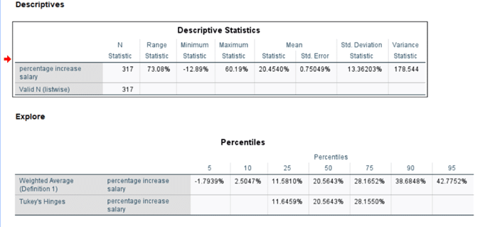
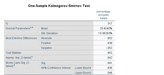
Kolmogorov-Smirnov test (52-62) – (Source: SPSS based on the database, 2020)
This table provides descriptive statistics for the percentage increase in salary for 317 individuals. Interpretation:
Salary changes range from –12.89% to +60.19%.
The average salary increase is about 20%.
A relatively large standard deviation (13%) shows substantial variation among employees.
The second table shows the results of a K–S test applied to the variable percentage increase salary to check whether the data follow a normal distribution.
Basic Information
N = 317
The test uses 317 observations.
Normal Parameters (Mean = 20.454%, Std. Deviation = 13.362%)
These are the parameters of the normal distribution the test compares your data to.
2. Most Extreme Differences
These numbers show how far your actual distribution deviates from a perfect normal distribution:
Absolute = 0.052 → The largest deviation
Positive = 0.038
Negative = –0.052
The absolute value (0.052) is the main test statistic.
3. Test Statistic
Test Statistic = 0.052
This number represents the maximum difference between the observed distribution and the normal distribution.
4. Significance (p-value)
Asymp. Sig. (2-tailed) = 0.042
Monte Carlo Sig. (2-tailed) = 0.041
99% Confidence Interval: 0.036 – 0.046
These values indicate the statistical significance of the test.
Interpretation of the p-value
The key decision rule:
If p > 0.05 → the data fit a normal distribution.
If p < 0.05 → the data do NOT fit a normal distribution.
Here:
p = 0.042 (asymptotic)
p = 0.041 (Monte Carlo)
Both are below 0.05.
In conclusion:
The Kolmogorov–Smirnov test indicates that the variable percentage increase in salary does NOT follow a normal distribution.
This means:
The distribution is not symmetrical.
It may be skewed (as earlier percentiles suggested).
You should be careful when using statistical tests that assume normality.
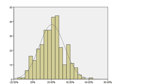
Normal distribution chart (52-62) – (Source: SPSS based on the database, 2020)
This histogram displays the distribution of the percentage increase in salary for 317 employees, along with a fitted normal curve (the smooth grey line). Overall, the histogram visually supports the statistical tests:
The data is not normally distributed (slight right skew).
There is a concentration around 20%.
A minority of employees received unusually high increases.
A few employees received salary reductions.
By using the graph, we can see that the distribution of salary increase percentage after standardize is not normal in the interval (52-62) and the graph, although it looks symmetrical, has some outlier data.
Q – Q chart (52-62) – (Source: SPSS based on the database, 2020)
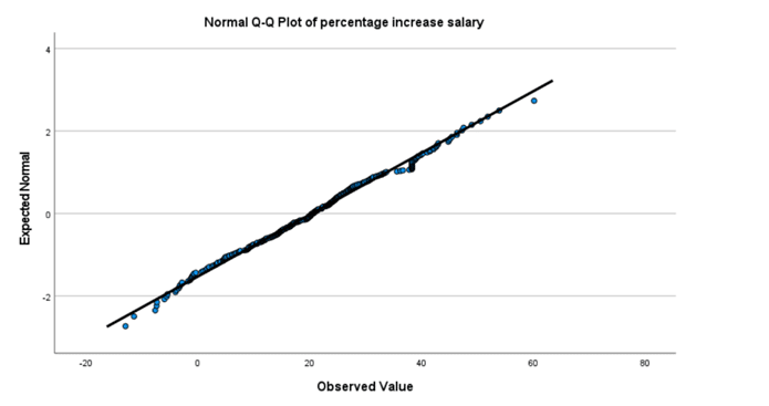
This Q–Q plot compares the observed salary increase values with the values expected from a perfect normal distribution. The Q-Q chart shows, on the horizontal axis the observed data and on the vertical axis the expected data. The distribution is normal if the observed data lie on or close to the line drawn from the corresponding quantiles. In the interval (52-62), the data at the beginning and middle of the chart are far from the drawing line. Overall, Even though the middle section of the data is fairly normal, the deviations in both tails especially the longer right tail mean that the percentage increase in salary does not follow a perfect normal distribution.
The distribution is positively skewed, with a few employees receiving unusually high raises.
Trend chart (52-62) – (Source: SPSS based on the database, 2020)
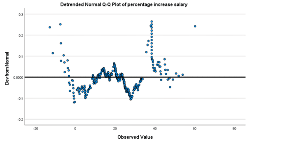
The detrended Q–Q plot illustrates the deviation of each data point from what would be expected under a perfect normal distribution. The horizontal line at zero represents exact normality; points above or below this line indicate deviations.
Overall Interpretation:
The detrended Q–Q plot shows that while the central portion of the salary increase data is somewhat normal, the tails especially the right tail deviate strongly. This indicates:
The distribution is positively skewed.
There are heavier-than-normal tails.
Outliers exist, particularly at high salary increases.
The variable does not meet the assumption of normality.
The trend graph shows the horizontal axis of the observed data and the vertical axis of the deviation from the normal distribution if the trend continues. The Y=0 line is a display tool for checking the deviation from the normal distribution. Any number of circles randomly placed around this line indicates a normal distribution. This graph shows that in the interval (52-62), if the trend continues, the data distribution around the mentioned line is not random, so the distribution is not normal.

P-Plot table (52-62) – (Source: SPSS based on the database, 2020)
The P-Plot table summarizes the parameters of the Normal distribution that has been fitted to the variable percentage increase in salary. Overall, while the average salary increase percentage in the period (52-62) is equal to 20.45, its standard deviation is 13.36. Standard deviation is an index to detect the amount of data dispersion around the mean and shows how far the data is from the mean value. It shows that the increases vary widely among employees, suggesting a high level of dispersion.
In terms of unweighted cases, each case (each employee’s salary increase) was given equal importance and no weighting adjustments were applied during estimation.
However, based on the Q–Q plot and detrended plot, this variable does not actually follow a normal distribution, even though the software provides estimated normal parameters. Thus, these parameters should be interpreted with caution.
In the main analysis published in the book, the Kolmogorov-Simonov test was performed and the results were similar and the data were non-normal in all groups. The general conclusion of these tests shows; Because the value of Sig or P-Value is less than 0.05, the test is significant. In other words, when the statistical population is not normal, the same formula cannot be used to change the conditions of that population.
Also, to check the increase percentage variable after standardize, you cannot use parametric tests such as t-test, regression, etc., and non-parametric tests such as chi-square, Friedman, Mann-Whitney Kruskal-Wallis, Jonker Terpstra tests should be used to check the effect of variables on each other. and use Wilcoxon.
-Is the frequency distribution of all educational levels the same?
One-sample chi-square test and frequency distribution test:
One of the non-parametric tests is chi-square test. This test shows the difference between observed variables and expected variables from a society. Also, in this section, I want to examine the abundance distribution in the educational levels of the retired community, and since there is no relationship about the classified variables and each one is independent, I used the chi-square test and the abundance distribution test. To perform this test, I first divided the educational qualifications into five classes and to identify them in SPSS software, I converted the qualitative variable into a class in the academic qualifications column.
Classification of educational qualifications of retirees:
1-Lower than ninth grade
2-Lower than diploma
3-Diploma
4-College graduate
5-Bachelor’s degree
6-Master’s degree
7-Ph.D
Now, I define zero and one assumptions as follows to display the percentage and frequency of educational qualifications of each time period:
H0: The frequency distribution of all education levels is the same.
H1: The frequency distribution of all educational levels is not the same.
The test of the second group, which are in the range (63-72):

One-sample chi-square test (63-72) – (Source: SPSS based on the database, 2020)
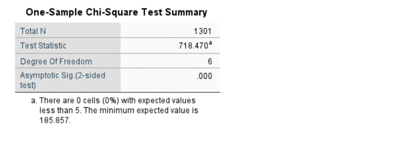
The table illustrates the significance level (p = 0.000) is less than 0.05, the result is statistically significant. Overall, There is a significant difference in the frequencies of the different education level categories.
In other words, the education levels do not occur with equal probability in the sample.
The distribution of education level is unequal, meaning some categories appear more (or less) frequently than others.
The null hypothesis that the distribution of the frequency of educational qualifications is the same in the interval (63-72) is rejected.
This is the calculated Chi-Square value comparing the observed frequencies with the expected equal frequencies.
Since p = 0.000 < 0.05, we reject the null hypothesis.
This means:
The distribution of education levels is not uniform.
Some education levels occur significantly more often (or less often) than would be expected if all categories had equal probabilities.
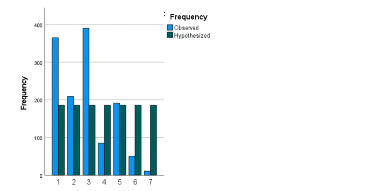
Classification test of educational qualifications (63-72) – (Source: SPSS based on the database, 2020)
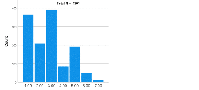
Degree distribution frequency test (63-72) – (Source: SPSS based on the database, 2020)
-Do the levels of educational qualifications have a significant effect on the percentage of salary increase?
This means the analysis is based on 1301 respondents, with only one missing value.
Percentiles
These values show the distribution of the variable (most likely education level or degree category based on the earlier context):
25th percentile: 1.00
50th percentile (median): 3.00
75th percentile: 4.00
This indicates:
25% of respondents fall at category 1 or below
50% fall at category 3 or below
75% fall at category 4 or below
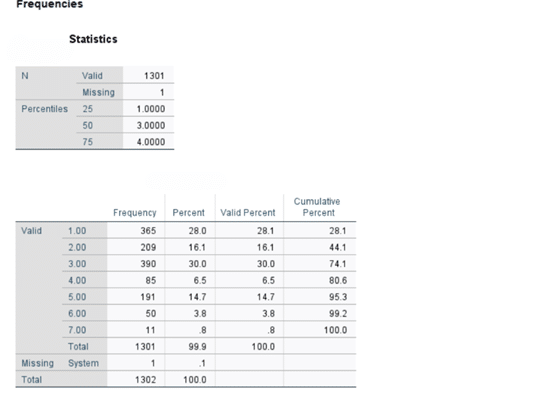
The highest frequency is related to diploma with the number of 390 people from the statistical population of 1301 people and 30% of the people, and then it is lower than ninth grade with the number of 365 people and 28% of the total population. The lowest frequency is related to PHD with the number of 11 people and 0.8%, and the rest of the degrees are: lower than diploma 16.1%, college graduate 6.5%, bachelor’s degree 14.7% and master’s degree 3.8% of the total population.
In the graphs drawn, we can also see the number of educational qualifications in comparison with each other and in comparison with the hypothetical value.
Frequency Distribution
This table shows how many respondents fall into each category (1 to 7):
Category Frequency Percent Valid Percent Cumulative Percent
1 365 28.0% 28.1% 28.1%
2 209 16.1% 16.1% 44.1%
3 390 30.0% 30.0% 74.1%
4 85 6.5% 6.5% 80.6%
5 191 14.7% 14.7% 95.3%
6 50 3.8% 3.8% 99.2%
7 11 0.8% 0.8% 100%
Interpretation
The most frequent category is 3 (30%).
The second most frequent is 1 (28%).
Higher categories (6 and 7) are rare (less than 4.6% combined).
This suggests the variable is positively skewed, with most respondents concentrated in the lower-to-middle categories.
From the interpretation of this test, we can conclude that the low percentage of salary increase after standardize, which is equal to 3.27% and having a diploma, as well as the high percentage of salary increase after assimilation, which is equal to 64.75% and having a lower than ninth grade, shows that the degree The education of people in the period (63-72) has not had a significant effect on the percentage of salary increase.
In the main analysis published in the book, this test was conducted for all groups and different results were obtained.
When scrutinized more rigorously, it can be concluded that the low percentage of salary increase after standardize, which is equal to 10.67% and having college graduate, as well as the high percentage of salary increase after standardize, which is equal to 90.51% and having PHD, shows that the educational qualification of the sacrifices group It has not had a significant effect on the percentage of salary increase. In the tests conducted in this section, it was shown that the degree score does not have a significant effect on increasing people’s salaries. It seems that this is one of the flaws of the model that should be paid more attention to that.
-Is there a significant difference in the average amount of benefits in different groups?
Kruskal-Wallis test and Janckheere – Terpstra test
The Kruskal-Wallis test is based on rank and is used to determine statistically significant differences between different groups. Janckheere – Terpstra test is also used to determine the existence of a statistical trend between independent and dependent variables sequentially or continuously. The difference between these two tests is that the Kruskal-Wallis test cannot predict the dependence of the dependent variable on the independent variable groups.
Both tests are alternatives to regression tests and one-way analysis of variance (ANOVA), which are used for parametric variables. It should be noted that these tests only determine whether there is a significant difference between variable groups, and to find out which group is superior, we must use the mean test.
I will do this test for the period (63-72) and to start the test, I will determine and group the dependent and independent variables and consider the assumptions of the test:
- Dependent variable (Y): Sum of standardize salaries
- Independent variables (X): Benefit salary with deduction of work experiences
(Management reward and overtime work)
To rank the independent variable, I classified the benefits into 5 groups:
1-Score between 4000 and 8000 first group
2-Points between 8000 and 12000 second group
3-Points between 12,000 and 16,000, third group
4-Points between 16,000 and 20,000, fourth group
5-Score 20,000 and above, fifth group
Test assumptions:
H0: The average amount of benefits in different groups is not significantly different.
H1: There is a significant difference in the average amount of benefits in different groups.

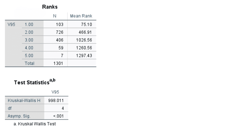
Kruskal-Wallis test (63-72) – (Source: SPSS based on the database, 2020)
Benefits:
N = 1301
The dataset contains 1,301 observations for this variable.
Mean = 2.3397
On average, the Benefits score is about 2.34, indicating a generally moderate level on the scale used (likely 1–5).
Std. Deviation = 0.71136
The standard deviation is relatively small, suggesting that responses do not vary widely around the mean.
Minimum = 1.00, Maximum = 5.00
The full range of the scale is represented.
Percentiles:
25th percentile: 2.00
Median (50th): 2.00
75th percentile: 3.00
Most values lie between 2 and 3, confirming low-to-moderate variability and a slightly right-skewed distribution.
V95:
A continuous variable with very high variance.
Large differences between minimum, maximum, and mean.
Distribution appears more uniform within the middle range (111M–146M).
-What is the trend of changes in benefits compared to changes in standardize salary?
The table shows the mean rank of variable benefits across five groups (1.00 to 5.00):
A higher mean rank indicates larger values in that group.
You can see a clear increasing pattern from group 1 to group 5
The Kruskal–Wallis H = 998.011 with df = 4 is very large.
The p-value < .001, meaning the result is statistically significant.
The result of the test shows that the Asymp Sig value is less than 0.05, the null hypothesis that there is no significant difference between the perks groups is rejected and there is no reason to confirm the null hypothesis. Interpretation of the Ranks table shows us the ranking of benefits groups based on their average. As can be seen, there is a significant gap between the groups.
In conclusion, there are significant differences among the five groups of benefits.
In other words, the distribution of benefits is not the same across groups.
Given the increasing mean ranks, it appears that higher group categories have substantially higher benefits values.
Now we perform Janckheere -Trepstra test for the same interval and above variables and assumptions:
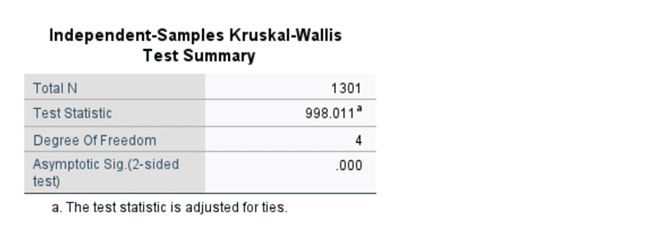
Janckheere – Terpstra test (63-72) – (Source: SPSS based on the database, 2020)
-Is there a significant difference in the average percentage increase in standardize between different occupational groups?
The table summarizes the results of the Kruskal-Wallis test, a non-parametric statistical test used to determine whether there are statistically significant differences between two or more independent groups on an ordinal or non-normally distributed variable.
1.Total N: 1301
This indicates that the total number of valid observations included in the test is 1,301.
2.Test Statistic: 998.011
The Kruskal-Wallis H statistic is 998.011.
A larger H value typically indicates greater differences between the groups.
3.Degrees of Freedom (df): 4
The degrees of freedom correspond to k − 1, where k is the number of groups.
Here, df = 4 → meaning 5 groups were compared.
4.Asymptotic Significance (2-sided test): .000
The p-value is < .001, which is highly significant.
In conclusion, Since p < .001, we reject the null hypothesis.
There is a statistically significant difference between the groups on the variable perks.
This means the median values (or distributions) of the groups are not equal, and at least one group differs significantly from the others.
As a result, the value of Sig is less than 0.05, so the null hypothesis is rejected, which means that there is a significant difference between the averages of the perks groups.
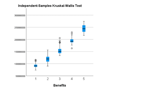
Janckheere – Terpstra diagram (63-72) – (Source: SPSS based on the database, 2020)
The boxplot visualizes the distribution of V95 (income/amount) across five levels of the variable “Benefits.”
1. Median values increase across benefit levels
Each box represents the distribution of V95 for a specific Benefits category (1 to 5).
The median (the line inside each box) rises steadily from Benefits = 1 to Benefits = 5.
This shows a strong positive relationship:
As perceived benefits increase, V95 (income/amount) also increases.
2.Distribution spreads widen for higher benefit levels
Higher benefits categories (4 and 5) show:
wider boxes (greater interquartile range → more variability)
longer whiskers
more outliers
This means:
People with higher benefit levels have a broader and more scattered distribution of benefits.
This graph shows that the trend between the dependent and independent variable is an increasing trend, considering that the overtime ceiling is considered for everyone, the smallest change in management rewards will increase the sum of standardize salaries.
Outliers are present but consistent with the pattern
The circles above some boxes indicate outliers.
However, even the outliers follow a consistent upward trend, reinforcing the positive association.
Visual pattern matches the Kruskal–Wallis statistical test
You previously obtained:
H = 998.011
df = 4
p < .001
This indicates:
The differences in V95 across benefit groups are statistically significant.
The boxplot visually confirms this:
Groups do not overlap much
Medians are far apart
Higher benefit levels clearly correspond to higher V95 values
Overall, the boxplot graphically supports the Kruskal–Wallis findings:
V95 values increase significantly and consistently with higher Benefits levels.
This means that:
Individuals who report higher benefits tend to have substantially higher V95.
The relationship is monotonic and strong.
The differences are both statistically significant and visually obvious.
In conclusion, this graph shows that the trend between the dependent and independent variable is an increasing trend, considering that the overtime ceiling is considered for everyone, the smallest change in management rewards will increase the sum of standardize salaries.
-Are the rankings of salary variables significantly different from each other?
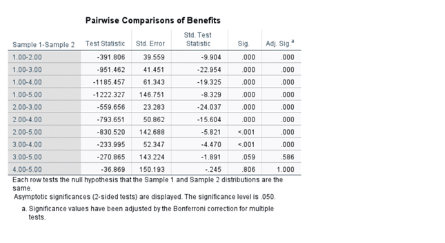
Comparing the average ranks of the two groups (63-72) – (Source: SPSS based on the database, 2020)
The table compares the average ranks of independent variable of two groups in (63-72). Overall, The smaller the value of Std.Test Statistic shows, the average rating distance is more meaningful. Looking at Adj.Sig in more detail, it corrects the type 1 error value and reduces the chance of false positives. As a result of this test, it is clear that all cases are zero and there is no type 1 error.
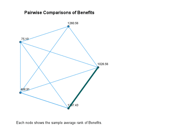
Comparing the ranks of the two groups (63-72) – (Source: SPSS based on the database, 2020)
The graph compares the sample average rank of benefits of the two groups in (63-72). The cases with significant difference show by light blue and the cases with no significant difference display by bold blue colors. There were the written numbers which are the average ranks specified in the Ranks table. From an overall perspective, there was a significant difference in groups one and two with group three and group five.
-What is the average benefits for different groups?
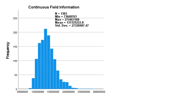
Frequency chart of benefits for different groups (63-72) – (Source: SPSS based on the database, 2020)
The histogram shows the distribution of the continuous variable average benefits for N = 1301 cases. From an overall perspective, the distribution is positively skewed (right-skewed):
Most observations cluster between 9,000,000 and 15,000,000.
A long tail extends to the right, reaching up to 27,446,316.
This indicates that: A small number of extremely high values pull the distribution to the right.
Looking at central tendency and distribution in more detail, the mean is 13,112,522. However, because of right skewness the mean is higher than the median (12,839,642 from earlier tables).
This difference confirms that extreme high values influence the average. In fact, median is more representative than the mean for this variable. The histogram demonstrates that benefits is not normally distributed but is right-skewed, with most values centered around 12–14 million and a small number of very high values extending the tail. In conclusions, the distribution is skewed, not symmetric. Median is a better central measure than the mean. High variability due to extreme upper values. Outliers exist but represent real variation rather than data errors.
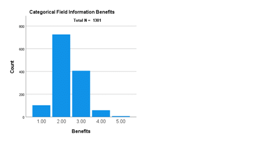
Frequency chart of people in different groups (63-72) – (Source: SPSS based on the database, 2020)
The graph shows the frequency of the number of people in different perks groups. In total, the Janckheere Terpstra test shows the existing trend between the independent variables and the dependent variable, in other words, it shows that the amount of more perks leads to an increase in standardize rights, and this increase has a significant difference between the existing groups.
-Difference in pension increase percentage according to job grouping
Mann-Whitney test
Mann-Whitney test is a non-parametric test and substitutes t-test for parametric tests. This test is used to compare the average of two groups of data. First, they rank the variables, then it is checked whether the ranks of the two groups are significantly different. What we want to address in this section is that; Is there a significant difference between the job groups in the organization in terms of the percentage of standardize salary increase or not? Considering that the job titles in the organization have changed over the years and finally in 1400, many job titles were removed and a total of 54 job titles were designed in 5 job categories, so the need to change and adapt these titles to the existing data was felt strongly.
Therefore, I manually changed all job titles in the initial data to new job titles; But in these changes, I did not include the job degree; Because it did not affect the analysis and only the job category was needed. Then I ranked the job categories as follows:
1-Headquarters and support jobs
2-Technical and engineering jobs
3- Programming jobs
4-News jobs
5-Maintenance and protection jobs
In the period (83-92), I want to repeat the Mann-Whitney test between the first group (headquarters and support jobs) and the third group (programming jobs):
Test assumptions:
H0: There is no significant difference between the average percentage increase in the standardize of the first group and the third group.
H1: The average percentage increase in standardize of the first group is significantly different from the third group.
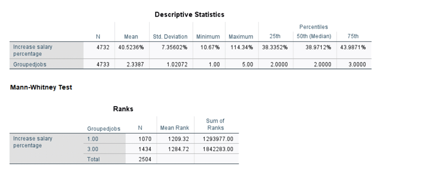
Mann-Whitney test (83-92) for the first and third groups – (Source: SPSS based on the database, 2020)
The table compares first group and third group of grouped jobs in the average percentage increase pensions. Overall, these values shows pensions increases cluster mostly between 38% and 44%. The distribution is somewhat right-skewed (maximum is much higher than the median). The median (38.97%) is a more robust indicator than the mean due to the extreme maximum value (114.34%).
Participants in job group 3 tend to have higher salary increase percentages than those in job group 1. The higher mean rank (1284.72 vs. 1209.32) shows the direction of the difference even before looking at the significance test.
The table illustrates the 4732 people in the statistical population in this period, 1070 people were identified as the first group and 1434 people were identified as the third group. The average of the staff and support occupations that make up the first group is lower than the average of the third group or the programming occupations group. In other words, the staff and support job group has an average of 1209.32 and has a lower average salary increase after standardize than the programming job group with an average of 1284.72.
Although the p-value is not shown in this screenshot, the rank difference is sizable.
Given is a table providing us with statistical information regarding large sample size (n = 2504 combined), there are the clear difference in mean ranks.
It is highly likely that the Mann–Whitney U test is statistically significant (p < .001).
In conclusion, there is a statistically significant difference in salary increase percentages between job group 1 and job group 3. Employees in Group 3 receive higher salary increases on average compared to Group 1.
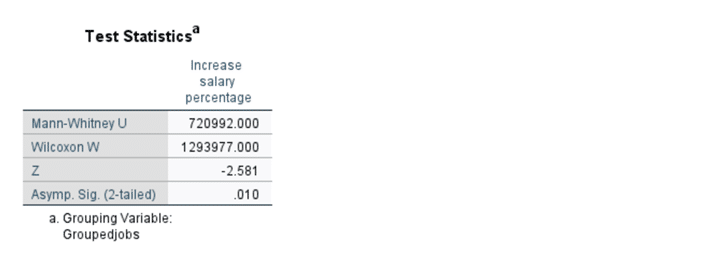
Test Statistics table of Mann-Whitney test (83-92) for the first and third groups – (Source: SPSS based on the database, 2020)
The table illustrates the Mann-Whitney test statistic is 720992 and the Sig value is 0.010, which is less than the significance level of 0.05. So the null hypothesis that “the average percentage of increase after standardize of the first group is not significantly different from the third group” is rejected. And the test shows that there is a significant difference between the first and third groups in the average percentage increase after standardize, and the third group has a higher average than the first group. Repeating this test in two time periods and rejecting the null hypothesis can bring us closer to the conclusion that the average salary increase percentage after standardize in the first group and the third group is different based on the statistical population.
Interpretation of the Z-score
The Z-value is: Z = –2.581
The negative sign indicates the direction of the difference:
Group 3 has higher salary increase percentages
Group 1 has lower salary increase percentages
This matches the rank table you showed earlier where:
Group 3 had the higher mean rank (1284.72)
Group 1 had the lower mean rank (1209.32)
In the main analysis published in the book, this test was conducted for all groups and different results were obtained.
-What is the average percentage of salary increase after standardize in different groups?
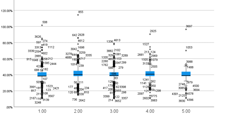
Box plot diagram (83-92) – (Source: SPSS based on the database, 2020)
The Box plot diagram compares five different job groups in (83-92) after standardize in term of the percentage of increasing pensions. Overall, the average of all groups is close to 40%, and group 2 and group 4 are slightly above the average compared to other groups.
When scrutinized more rigorously, it can be concluded that, the average percentage of increasing pensions after standardize in different groups is different based on the statistical population, Following a similar pattern, the average of group 2 and 4 are higher than other groups slightly. What stands out more than anything else is the number of outliers and outliers in the model, which we will discuss in the next sections.
-Is there a significant difference in adding the matching difference score in the final standardize retirement score?
Wilcoxon test
The Wilcoxon test is one of the non-parametric tests used to measure the similarity of two dependent samples with a rank scale. In this test, it is possible to compare the size of the difference between the ranks before and after the implementation of a plan. This test corresponds to the paired t test in the normal statistical population. In addition to the direction, the Wilcoxon test tests the size of the difference between similar groups. As mentioned in the database section, the final standardize pension score, which is one of the standardize rights items, is calculated from the following formula:
Adjustment difference score + retirement score by applying the years’ deduction factor.
Using the Wilcoxon test, we want to check how much the final standardize pension score is different before and after the matching difference score is added. Therefore, we define the assumptions of the test as follows:
Test assumptions:
H0: There is no significant difference between the addition of matching difference score in the final standardize pension score.
H1: Adding matching difference score has a significant difference in the final standardize pension score.
To rank the match difference score, I classified it into 4 groups:
1-Score between 9000 and 35.000 first group
2- Points between 35,000 and 60,000 of the second group
3- Points between 60,000 and 85,000, third group
4- Points between 85,000 and 110,000, fourth group
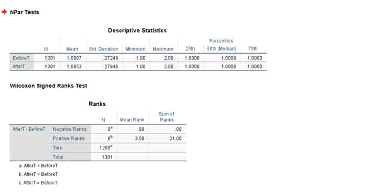
Wilcoxon test (63-72) – (Source: SPSS based on the database, 2020)
This test checks whether there is a significant difference between BeforeT and AfterT for the same subjects. In the interpretation of the test result, we can see that in the range (63-72) with the number of 1301 people in the statistical population, the average negative rating is zero and the average positive rating is 3.5. In other words, the final standardize pension score after adding the matching difference score is higher than before adding it. This means that the final standardize pension score has improved.
However, statistical significance must be interpreted carefully because the number of actual changes is extremely small:
Positive ranks: 6
Negative ranks: 0
Ties: 1295
This means only 6 out of 1301 participants showed improvement, and 1295 showed no change.
The statistical significance is driven by the test’s sensitivity to even a very small number of changes in a large sample.

Wilcoxon test statistics table (63-72) – (Source: SPSS based on the database, 2020)
The Z test statistic is equal to -2.449 and is significant at the 0.014 level, and the null hypothesis that “adding the matching difference score the final standardize pension score has no significant difference” is rejected. In fact, there is a significant difference between before and after adding the match. Even though the test shows a statistically significant difference between Before T and After T:
The practical (real-world) difference is extremely small.
The means differed only slightly:
- BeforeT Mean = 1.0807
- AfterT Mean = 1.0853
This change is not meaningful in practical terms.
In the main analysis published in the book, this test was conducted for all groups and different results were obtained.
The adjustment difference amount is one of the negative items in the employee’s salary, which if removed, the employee’s salary will increase. The Wilcoxon test leads us to the conclusion that in this plan, adding the matching difference score to the final standardize pension score will lead the lower income level to the matching difference score, which has a negative effect on salaries and does not bring a good result.
-Are the ranking of the independent salary variables different from each other significantly?
Friedman test
Friedman’s test is one of the non-parametric and generalized Wilcoxon tests for non-normal variables. This test is used to rank or prioritize variables. In this part, we want to measure the ranking of the items affecting pension after standardize.
To conduct the test, I select the statistical population from the period (93-99) and define the standardize as follows:
Test assumptions:
H0:The ranking of the independent salary variables are not significantly different from each other.
H1:The ranking of the independent salary variables are significantly different from each other.
The salary items that we want to evaluate are:
A-The final score of standardize pension
B-Amount of job scores with deduction of years of work experiences
C-Amount of related to the work place scores with deduction of years of work experiences
D-Perks score with deduction of work experiences
For each of the above points that make up the independent variables, based on the lowest to the highest score, I did the ranking as follows:
A-The final score of standardize pension:
1-Score between 16000-23000 first group
2-Score between 23000-30000 second group
3-Score between 30,000-37,000, third group
4-Points between 37000-44000, fourth group
5-Score 44,000 and above, fifth group
b-Amount of job scores with deduction of years of work experiences:
1-Score between zero-1000 first group
2-Score between 1000-2000 second group
3-Score between 2000-3000, third group
4-Score between 3000-4000, fourth group
5-Score 4000 and above, fifth group
C-Amount of related to the work place scores with deduction of years of work experiences
1-Score between zero-700 first group
2-Score between 700-1400 second group
3-Score between 1400-2100, third group
4-Score between 2100-2800, fourth group
5-Score 2800 and above, fifth group
D-Perks score with deduction of work experiences:
1-Score between 4000 and 8000 first group
2-Points between 8000 and 12000 second group
3-Points between 12,000 and 16,000, third group
4-Points between 16,000 and 20,000, fourth group
5-Score 20,000 and above, fifth group
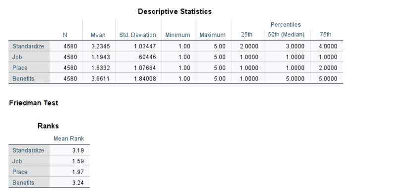
Friedman test (93-99) – Source: SPSS based on the database, 2020)
According to the conducted test, in the Median section of the descriptive statistics table, it can be seen that the median score of perks is equal to 5 and higher than the other scores, and the median job additional amount scores and work place additional amount scores is equal to one.
The table shows the ranking of the independent variables. The perks score has the highest rank and is equal to 3.24, followed by the standardize score with a rank of 3.19. There is a slight difference in the ranking of job additional amount scores and work place additional amount scores, which work place additional amount scores is higher with a rating of 1.97. Although the image does not include the chi-square value and p-value, the Friedman test will definitely be significant (p < .001) with:
Extremely large sample size (N = 4580)
Clear rank differences (1.59 → 3.24)
So you can safely report:
The Friedman test showed a statistically significant difference among the four dimensions.
A Friedman test was conducted to compare scores across four related dimensions (Standardize, Job, Place, Benefits). The test revealed a statistically significant difference among the groups, χ²(df = 3) = [SPSS value], p < .001. Mean ranks indicated that Benefits (MR = 3.24) and Standardize (MR = 3.19) received the highest evaluations, while Place (MR = 1.97) and Job (MR = 1.59) were rated significantly lower. These results suggest substantial differences in how respondents perceive these four dimensions, with Benefits being the most positively evaluated.
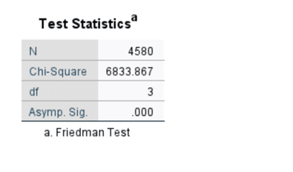
Friedman’s test statistics table (93-99) – (Source: SPSS based on the database, 2020)
The Test Statistics table shows that in the statistical population with the number of 4580 people and the degree of freedom of 3, the Sig value is equal to zero and is less than the significance level of 0.05. So, the null hypothesis that “rankings of independent salary variables are not significantly different from each other” is rejected and there is a significant difference between the ranks of the independent variables that make up pension items. The Friedman test helps us to focus on the items that have a greater impact on pension and to improve them.
There is a statistically significant difference among the four variables.
The ratings of the four dimensions (Standardize, Job, Place, Benefits) are not equal.
Given the very large chi-square value (6833.867), the differences are highly significant and substantial.
-Clustering pensions by their increasing percentage.
Clustering
Clustering is a method in which objects are grouped based on qualitative and quantitative characteristics. This operation is done with the highest similarity in each cluster and the lowest similarity between clusters. There are different types of clustering, the selection of which is based on the type, volume and number of data. In this section, we want to cluster standardize pension as well as salary increase percentage. For this purpose, we use discriminative clustering or K-means. In this type of clustering, K cluster centers are randomly selected and the distance between each point and the cluster center is calculated. And it is formed based on the smallest distance between the points to the center of the cluster. In this test, we consider K=4.
For the interval (73-82), we perform K-average clustering for standardize pension and pension increase percentage:
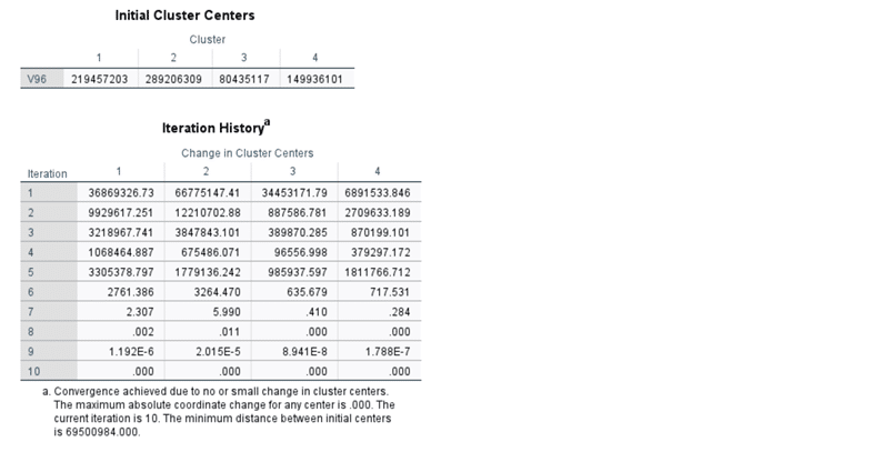

Clustering K-means Standardize pension (73-82) – (Source: SPSS based on the database, 2020)
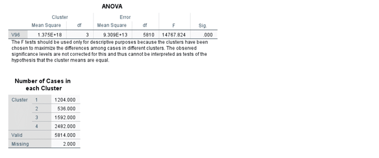
ANOVA table and frequency of income clusters (73-82) – (Source: SPSS based on the database, 2020)
The table labeled “Initial Cluster Centers” shows the starting values for each cluster (1 to 4) based on variable average standardize pension.
These are very large numerical values, which suggests that:
- The variable being clustered is likely a large-scale measurement (e.g., population, revenue, cost, or another metric measured in large units).
- K-means begins with these four initial seeds as the starting positions for each cluster.
The test result shows that the clustering process is done in 10 steps until there is no more change in the clustering centers. Finally, 4 clusters have been created with the following average centers:
Cluster 1: with an average center of 165,191,106 Rials
Cluster 2: with an average center of 204,214,158 Rials
Cluster 3: with an average center of 112,835,647 Rials
Cluster 4: with an average center of 137,492,433 Rials
In the Number of Cases in each Cluster table, the number of members in each cluster is shown, which according to the results, cluster 4 with the number of 2482 people out of 5814 people from the entire statistical population and the average standardize pension of 137,492,433 Rials is the largest number and cluster 2 with 536 people and the average The standardize pension have the lowest number of 204,214,158 Rials.
Clusters Represent Four Distinct Levels
The values of average standardize pension are very large, and the clustering algorithm has separated them into four groups, ranging from the lowest to the highest:
Cluster 3: Lowest salary increase percentage values (~112M)
Cluster 4: Lower-middle values (~137M)
Cluster 1: Upper-middle values (~165M)
Cluster 2: Highest values (~204M)
This ordering indicates a gradient-based clustering, where the model detected natural breaks in the magnitude of average standardize pension.
ANOVA Results illustrate that very large F-value (14767.824)
Indicates extremely strong differences between the cluster centers on variable average standardize pension.
Significance level (Sig = .000)
Although SPSS notes that this significance value should only be used descriptively (because K-means maximizes cluster separation), the result still shows:
The clusters differ dramatically in terms of average standardize pension. Average standardize pensionis an important variable for distinguishing the groups. High between-cluster variance (1.375E+18)
This shows that the variable average standardize pension explains a large portion of the separation among clusters.
Very low within-cluster variance (9.309E+13)
Indicates that items inside each cluster are relatively similar to each other compared to other clusters.
In conclusion, the clusters are clearly and strongly differentiated based on average standardize pension, which validates the clustering model.
Now, in the same period, we perform clustering for the pension increase percentage after standardize:

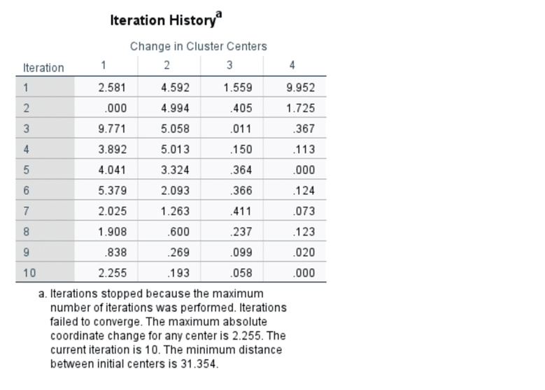
K clustering – average percent increase (73-82) – (Source: SPSS based on the database, 2020)


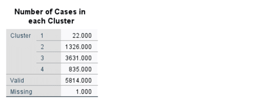
ANOVA table and frequency of percentage clusters (73-82) – (Source: SPSS based on the database, 2020)
The table shows the starting points for the K-means clustering algorithm, based on the salary increase percentage variable. These initial centers represent the starting estimates for four distinct groups of employees based on how much their salary increased.
Cluster 1 – Very High Salary Increase (≈106%)
This group has extraordinarily high salary increases, more than doubling their previous salary.
Represents employees who received exceptional adjustments (e.g., promotions, reclassification, special adjustments).
Cluster 2 – High Salary Increase (≈73%)
Employees in this group received large raises, well above typical increments.
Could indicate substantial performance-based increases or retention adjustments.
Cluster 3 – Moderate Salary Increase (≈41%)
This group received moderate increases.
Represents standard salary growth (e.g., annual adjustments, moderate merit increases).
Cluster 4 – Low Salary Increase (≈10%)
Employees here received small or minimal salary increases.
Likely represents standard cost-of-living adjustments or cases with limited salary progression.
In conclusion, the dataset contains four distinct behaviors in salary growth, ranging from minimal increases to extremely large jumps. The distribution suggests strong salary inequality or differentiation across employees. The cluster structure shows that employees are not receiving uniform increases; instead, there are very clear tiers.
The test result shows that the clustering process is done in 10 steps until there is no more change in the clustering centers. Finally, 4 clusters have been created with the following average centers:
Cluster 1: with an average center of 31.72%
Cluster 2: with an average center of 21.45%
Cluster 3: with an average center of 52.38%
Cluster 4: with an average center of 78.21%
The table shows how much the cluster centers changed during each iteration of the K-means algorithm. The values represent the movement (distance) of each cluster center between iterations. Key Observations from the Table
Iteration 1 shows relatively noticeable changes, especially for Cluster 4 (9.952) and Cluster 2 (4.592).
This is normal: in early iterations, cluster centers typically shift more.
In later iterations (6 to 10), the changes become very small.
Most values approach 0.0, meaning the algorithm is trying to stabilize.
The maximum center movement in the last iteration is 2.255, which is still above zero.
This means the algorithm did not reach perfect convergence.
The number of members in each cluster shows, which according to the results, cluster 3 with the number of 3631 people out of 5814 people from the entire statistical population and the salary increase percentage after standardize is 38.52%, the largest number and cluster 1 with 22 people and the salary increase percentage after standardize is 72.31%, the lowest number.
The final cluster centers represent the average salary-increase percentage for each of the four employee groups identified by the K-means clustering algorithm. These clusters highlight meaningful differences in compensation growth across the workforce and can guide strategic decision-making.
Cluster 1 – High Salary Growth (72.31%)
This group has experienced the highest salary increase.
From a managerial perspective, this cluster likely includes top performers, key talent, or employees in critical roles where retaining expertise is essential.
Cluster 2 – Moderately High Salary Growth (45.21%)
Employees in this group receive a solid, above-average salary increase.
They may represent consistent performers or individuals whose roles have moderate strategic importance.
Cluster 3 – Moderate Salary Growth (38.52%)
This group receives a lower-middle salary increase.
It likely includes employees with average performance or those in roles where compensation adjustments are more standardized.
Cluster 4 – Low Salary Growth (21.78%)
This cluster has the lowest percentage increase and may include underperformers, newly hired employees, or positions with limited budget allocation.
Overall, the clustering results reveal a clear segmentation of employees based on salary increase percentages:
High performers receive distinctly higher increases.
Middle groups show moderate differentiation, suggesting opportunities for improved performance-based reward alignment.
The lowest-increase cluster requires managerial attention to prevent morale issues or skill gaps.
These insights enable management to:
Strengthen compensation fairness and transparency
Improve performance management systems
Align salary policies better with organizational goals
Identify groups needing retention strategies or developmental support
Key Managerial Insights
1. Salary increases are not evenly distributed across employee groups
The very large F-value and extremely small p-value indicate that the differences between the clusters are substantial. This means employees fall into clearly distinct compensation-growth categories.
2. The organization uses differentiated salary-increase strategies
The clusters represent four distinct salary-growth patterns. Such variation suggests that the organization adjusts salaries based on:
performance levels
role criticality
seniority or tenure
strategic priorities
budget allocation policies
This confirms that the compensation system is not uniform, but rather targeted and differentiated.
3. The differences between clusters are meaningful and should be reviewed for fairness and alignment
Because clusters differ strongly, managers should:
Ensure that salary-increase policies are transparent
Verify that high-increase groups correspond to high performance or essential roles
Check whether employees with low increases (Cluster 4) risk disengagement or turnover
Evaluate whether the middle clusters require clearer performance criteria or development paths
4. Supports strategic workforce segmentation
The strong statistical separation reinforces that employees can be grouped into distinct salary-growth categories. This helps management:
Identify top-talent groups
Detect potential under-rewarded or high-risk groups
Plan targeted retention programs
Improve compensation fairness and long-term planning
The distribution of employees across the four salary-increase clusters is highly uneven.
1. Cluster 3 represents the majority of employees
With 3,631 employees, Cluster 3 is the dominant group.
This indicates that the salary-increase pattern of Cluster 3 reflects the typical or most common compensation behavior in the organization.
Managers should treat Cluster 3 as the baseline group for policy evaluation.
2. Cluster 1 is extremely small and likely represents an exceptional or special category
Cluster 1 includes only 22 employees, suggesting that this group may consist of:
top performers receiving unusually high increases
employees with unique roles or critical responsibilities
outliers due to exceptional circumstances
This group requires individual-level managerial review, not broad policy changes.
3. Cluster 2 and Cluster 4 reflect medium-sized segments with distinct salary-increase behaviors
Cluster 2 (1,326 people) forms a large secondary group, likely representing employees with moderately above-average increases.
Cluster 4 (835 people) represents another meaningful segment, potentially those receiving the lowest salary increases.
These two groups should be monitored for:
fairness
alignment with performance and role expectations
potential retention risks (especially Cluster 4)
4. Workforce segmentation is effective and meaningful
The significant variation in group sizes shows the clustering method successfully identifies real salary-increase patterns, not random noise.
This provides a reliable foundation for:
designing compensation strategies
identifying high-risk or high-value employee groups
planning differentiated HR interventions
Sometimes, two-stage clustering is used to cluster large data. This type of clustering automatically determines the number of clusters and the system considers a likelihood function and sets a comparison scale. In fact, a type of random sampling takes place, and it is assumed that the members of a sample who are selected, other members also have the chance of this selection, and the selection of members will not affect the other. We perform two-step clustering with these descriptions:
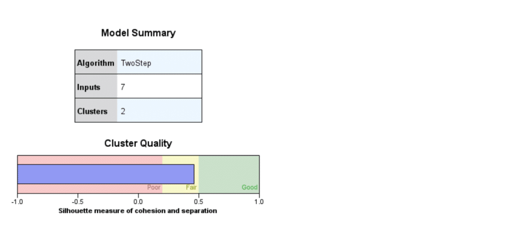
Two-stage clustering of percentage increase (73-82) – (Source: SPSS based on the database, 2020)
Based on the clustering result, we can see that the system created a cluster based on the likelihood function, which if we consider the measurement on a scale of -1 to +1, from -1 to +0.2 of the sample in the weak part, from +0.2 to +0.5 in the weak part. Average and from +0.5 to +1 are in the good part. According to the two-stage clustering, the observations in this interval are in the weak to moderate part.
The Two-Step clustering algorithm was applied using 7 input variables, and the model automatically identified 2 distinct clusters within the data.
This indicates that the underlying patterns among the variables naturally group into two meaningful employee segments.
Further refinement may be possible
If needed, managers could improve clustering quality by:
- Adding more predictive variables
- Reducing noise variables
- Running segmentation on subgroups (e.g., by job role or region)
- Standardizing numerical inputs
But for most purposes, the current model offers useful and actionable segmentation.
In the main analysis published in the book, income and percentage clustering for other groups was also done and analyzed.
In general, it can be concluded that the clusters are not similar and cannot be placed in the same groups. The average standardize pension for large clusters is about 132 to 137 million Rials and the average percentage increase for large clusters is 38 to 39 percent.
-If the model has outliers, how can they be identified and corrected?
Outlier data
Outliers are data that are far from the average of all data in a statistical population. Outliers do not behave as expected; They are like noise. Outlier data are not included in any cluster in data clustering, or even if they occupy a separate cluster due to the high percentage, they impose a lot of cost on the system and complicate the model. Outlier data change the shape of a statistical population from normal to abnormal. The presence of a small number of outliers in any model is inevitable and can be overlooked; But the concern starts from the fact that a large percentage of the population is made up of extraneous data that must either be deleted or corrected. From the results of the tests that were done in the previous parts, it seems; Our statistical population is abnormal due to the presence of outlier data. In this section, we want to identify outliers in the existing model and how to deal with them. In the previous part, we focused on clustering in the time period (73-82) for the percentage increase in standardize. In this part, we want to identify outlier data clustering from the result, and once again 4 clusters are created and we see the number of people in it. We also concluded that the highest number was observed in cluster 3 with a 38.52% increase. Now let’s draw a box plot to see outlier data:
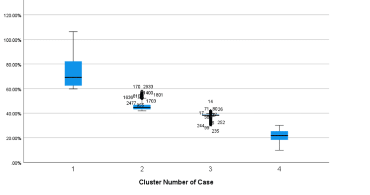
Boxplot diagram of percent increase and outlier data (73-82) – (Source: SPSS based on the database, 2020)
The boxplot illustrates the distribution of percentage values across four customer clusters. The clusters show distinct behavioral patterns, allowing managers to differentiate strategies for each group.
Cluster 1 – High-Value / High-Variation Segment
This cluster exhibits the highest median percentage (around 70%) and also a wide variability among its members. This indicates a segment with strong potential but inconsistent behavior.
Managerial insight: Tailored engagement and personalized follow-ups can stabilize and potentially increase their contribution.
Cluster 2 – Mid-to-High Stable Performers
Cluster 2 has a moderately high percentage (≈45–50%) with very low dispersion, reflecting stable and predictable behavior.
Managerial insight: This reliability makes them ideal for long-term programs, loyalty initiatives, and efficiency-oriented planning.
Cluster 3 – Mid-Level but Irregular Segment
This group shows percentages around 30–35%, but with visible outliers. Such irregularities suggest that a minority behaves very differently from the rest.
Managerial insight: Identify and analyze the outlier cases to determine whether they represent risk, emerging opportunities, or data anomalies.
Cluster 4 – Low-Value Segment
Cluster 4 has the lowest median (≈20%), with a narrower spread overall.
Managerial insight: This segment may require cost-effective strategies, automation, or re-evaluation of resource allocation. Upselling potential is limited but possible with targeted intervention.
As can be seen, the second and third clusters, which have the highest frequency of the community in which they are located, have many outlier data that are not included in the cluster. Circles on the graph marked with numbers are population outliers. According to the results of 291 outlier data, it has been shown that these numbers are higher or lower than the expected percentage of the society. The system has approximately considered the average percentage of community growth as 37.76 and measured it in relation to it.
In order to identify outlier data, according to the average percentage increase that is 37-38%, 10% of the upper level and 10% of the lower level can be considered; In other words, above 47% and below 27% can be considered as outlier data. Based on this, the number of outliers in each interval was identified and the result was as follows:
- In the interval (52-62), the number of 235 variables out of 317 numbers of the total statistical population equal to 74% are outlier data.
- In the period (63-72), 518 variables out of 1301 total statistical population equal to 40% are outlier data.
- In the interval (82-73), the number of 1037 variables out of 5814 numbers of the total statistical population equal to 18% are outlier data.
- In the interval (83-92), 783 variables out of 4732 numbers of the total statistical population equal to 16.20% are outlier data.
- In the period (93-99), the number of 1219 variables out of 4580 numbers of the total statistical population equal to 26.62% are outlier data.
- In the martyr sheet, 97 variables out of 526 numbers of the total statistical population equal to 18.44% are outlier data.
- In the total statistical population with the number of 16,744 variables, the number of outlier data is equal to 3,792 numbers, which constitute 22.64% of the total statistical population.
Analytical dashboards
Dashboards allow us to visualize multiple analyzes side by side in the form of different graphs. They also make it easier to compare and evaluate the results and give the analyst the opportunity to evaluate the advantages and disadvantages of the model and try to solve the problems by putting together different aspects of the analysis.
In the main analysis that was published in a book, this section includes two parts of veterans and non-veterans, each of which is divided into two parts: retired employees and retired managers. I have evaluated legal items using Excel and Power BI software, and I have designed analytical dashboards by selecting some random samples. But I briefly present three of the dashboards.
Non-veterans
Choosing a smaller statistical population from the main statistical population helps us to analyze by more detail. In this section, due to the large number of non- veterans retirees, I randomly selected a number from each interval and stored a total of 1000 non- veterans retirees in a separate sheet. This sheet includes managers and non- veterans retired employees.
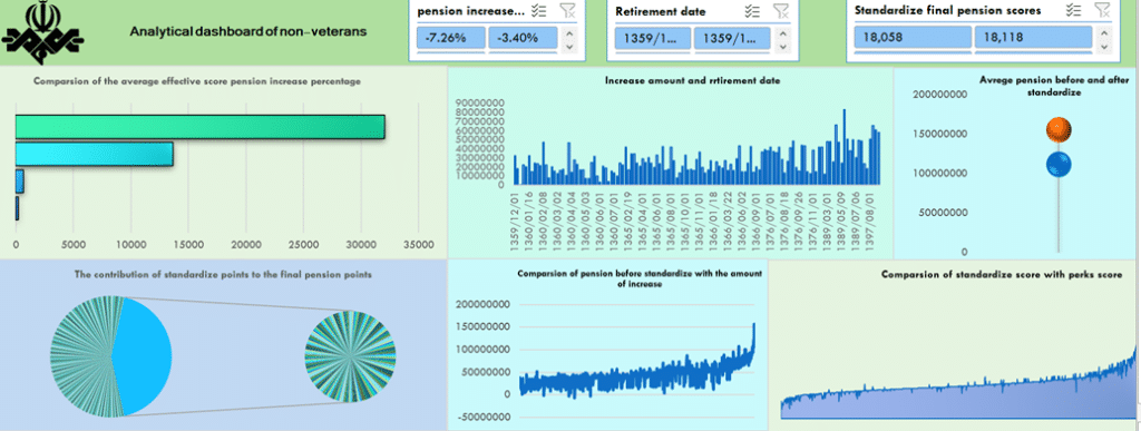
Analytical dashboard of the pensions of non-veterans – (Source: Excel based on the database, 2020)
-Average salaries before and after standardize for non- veterans’ employees?
- The candy chart illustrates the selected statistical population of 1000 people, the blue circle, which indicates the salary before standardize, is in the range below 100 million Rials to between 100 and 150 million Rials, and the orange circle, which indicates the pension after standardize, is in the range below 150 million Rials and between 150 and is 200 million Rials.
- -The effect of retirement date on the rate of increase in non- veterans’ employees.
- The graph shows that in the selected statistical population of 1000 people, apart from the outliers that exist in all years, the retirement date has no effect on the increase amount and is not among the effective items in pension increase.
- -Average effective points in the percentage of salary increases for non- veterans’ employees
- In the statistical population of 1000 selected people of veterans’ employees. Overall, the biggest share in the pension increase percentage is the standardize score and then the perks score. The work place additional amount is with a slight difference more effective than the amount job scores.
- -Comparison of the difference of matching score and benefit score
- Since the standardize score includes the difference of matching and work experiences, the small or large number of these items has a significant effect on the percentage of pension increase of individuals.
- –Comparison of pre-standardize salaries and increase amounts for non- veterans’ employees.
- In the statistical population of 1000 selected people of veterans’ employees. Overall, the average pension increase is below the line of 50 million Rials and up to 50 million Rials. Although in some parts we see an increase (decrease) below zero and an increase of up to 150 million Rials.
- –Comparison of the contribution of standardize points to the final retirement points for non- veterans’ employees
- The diagram illustrates the selected statistical population of 1000 people of veterans’ employees. The larger circle, which is the final retirement score, has allocated more than half of its score to the standardize score.
-Details of changes before and after standardize for non- veterans’ employees.
Using the above dashboard; It is possible to compare the effect of different factors on one page side by side. This dashboard is designed in Excel software and is dynamic so that the charts change by changing the slicer filter on the top of the screen. Also, the following items have been extracted from the analysis pension of non-veterans in the selected statistical population of 1000 people:
- The lowest percentage of increase (decrease): (-5.92%)
- The highest percentage increase: 85.20%
- Lowest income before standardize: 59 million rials
- Highest income before standardize: 292 million rials
- Lowest income after standardize without non-continuous the amounts plus and perks: 56 million Rials
- The highest income after standardize without non-continuous the amounts plus and perks: 311 million Rials
- Lowest income after standardize with non-continuous the amounts plus and perks: 72 million Rials
- Highest income after standardize with non-continuous the amounts plus and perks: 446 million Rials
- The percentage of outlier data in increasing the pension of non-veterans is 18%.
The last item is not shown in the dashboard above; But it has been checked in the preliminary calculations.
Veterans retired managers
From the information of 526 veterans of the organization, I extracted the information of 61 veterans and registered them in a separate sheet. This was done in order to take a more detailed look at the legal items of veterans retired managers.
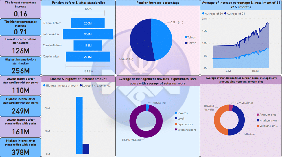
Analytical dashboard of the pension retired managers of veterans – (Source: Power Bi based on the database, 2020)
-Comparison of salaries before and after standardize of veterans’ managers in Tehran and Qazvin
- I randomly selected two level five general managers with doctorate degrees and the job titles of hardware and network engineer and information technology engineer from Tehran and Qazvin to compare their salaries before and after standardize. Funnell’s diagram shows salaries before and after standardize of veterans’ managers in Tehran and Qazvin. There was a difference of 21 million Rials in the salaries of the director of Tehran before and after standardize, the salary difference reached 37 million Rials.
-Comparison of the percentage of salary increases for veterans’ managers in Tehran and Qazvin
- The pie chart shows the percentage of salary increases for veterans’ managers in Tehran and Qazvin .Although the initial conditions of both people are apparently the same, the pension increase percentage of Tehran manager is 48.60% and Qazvin manager is 54.93%. Considering that the veterans’ manager of Qazvin is eligible to receive extras from work place additional amount, but other parameters such as experiences of management can be effective in this difference.
-Is the amount of salary increase and the share of installment payments suitable for veterans’ managers?
- The graph illustrates comparison of increase amount and monthly installments for veterans’ managers. Overall, At the lower level of the increase, the amount of installments is not proportional to the amount of increase and they are almost equal; But as it is added to the increase amount, it becomes a little more balanced. But in general, the average amount of installments seems high.
-Which of the items have a higher average in the salaries of veteran’s managers; final standardize salary, management amount and amount veterans ?
- The pie chart illustrates the average of amount veterans and the others average scores. In general, minimum amount of increase is about 20 million Rials and the maximum amount of increase is about 120 million Rials. The gap between these two amounts is one of the points that should be paid attention to. Overall, the self-sacrifice score is more than 96.85% and the reward, level and experiences of management scores make up 3.1% of the total.
-Comparison of average reward scores, experience, and management level, and veterans score in the salaries of veteran’s managers.
- The pie chart shows, comparison of average reward scores, experience, and management level, and veterans score in the salaries of veteran’s managers. Overall, the greatest effect in increasing the pension of retired managers is between standardize final pension scores and the management amount plus, the pension of veterans is related to the pension of veterans with 48.44% and then the standardize final pension scores with 47.5%. The share of management amount plus is 4.06%, which of course are calculated on average veterans pension are slightly higher than standardize pension.
This dashboard, which is designed with PowerBI software, is dynamic and can be changed by changing the initial data and gives us an overview of the summary of the analysis and the status of the plan in this section. On the left side of the dashboard, there are cards designed to depict the highest and lowest pensions and percentage increases for veterans retired managers.
-Details of changes before and after standardize of veteran’s managers.
- Lowest percentage increase: 16%
- The highest percentage increase: 71%
- Lowest income before standardize: 126 million Rials
- Highest income before standardize: 256 million Rials
- Lowest income after standardize without non-continuous amount plus and perks: 110 million Rials
- The highest income after standardize without non-continuous amount plus and perks: 249 million Rials
- Lowest income after standardize with non-continuous amount plus and perks: 161 million Rials
- Highest income after standardize with non-continuous amount plus and perks: 378 million Rials
- The percentage of outlier data in pension increase of veterans retired managers is 51.61%.
- The last item is not shown in the dashboard above; But it has been checked in the preliminary calculations.
Non-veterans retired employees
Among the 1000 selected people; 200 managers and 800 retired employees were stored in separate sheets. which was done in the previous part of the analysis of non- veterans retired managers. In this section, we randomly compare the information of two non- veterans retired employees who have similar conditions in terms of job titles and educational qualifications, and one of them is in Tehran and the other is in the provinces. An attempt has been made to select samples from every job category and to some extent from the last job levels. This comparison is selected for two specific people, and although it cannot be generalized to other people, it can give us a general view of the legal changes of these people.
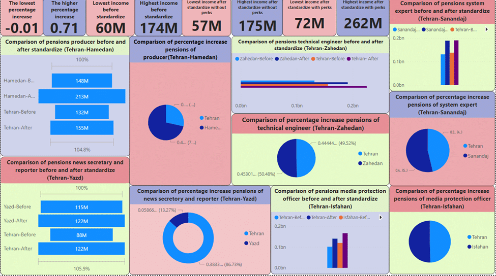
Analytical dashboard of pension non- veterans of retired employees – (Source: Power Bi based on the database, 2020)
–Comparison of salaries before and after standardize and the percentage increase in salaries of radio and television producers in Tehran and Hamada for non-veterans employees.
- The pie chart illustrates comparison of the percentage increase in salaries of radio and television producers in Tehran and Hamadan. The chart shows comparison of salaries before and after standardize. I chose a radio producer with a bachelor’s degree from “Tehran” and a television producer with a master’s degree from “Hamedan”, both of whom are in the professional master’s degree. The producer of “Hamedan” will receive more pension than the producer of “Tehran” with a pension difference of 58 million rials. It is worth noting that the pension of the producer of “Hamedan” was 16 million Rials more before the standardize. The percentage of pension increase of the producer of “Tehran” is 17.59% and the percentage of pension increase of the producer of “Hamedan” is 44.35%.
-Comparison of salaries before and after standardize and the percentage increase in salaries of technical engineerin Tehran and Zahedan for non-veterans employees.
- The bar chart shows salaries before and after standardize of technical engineerin Tehran and Zahedan. The pie chart illustrates comparison of the percentage increase in salaries of technical engineerin Tehran and Zahedan. From the technical and engineering jobs, I chose the job of technical engineer or hardware and network engineer in the new job titles. The technical engineer of “Tehran” has a bachelor’s degree and a senior professional degree, and the technical engineer of “Zahedan” has a master’s degree and a professional degree of 5. The technical engineer of “Tehran” will receive 34 million Rials more pension than the producer of “Zahedan” due to the legal difference. It is worth mentioning that the pension of the producer of “Zahedan” was 24 million Rials lower before the standardize. The percentage of pension increase of technical engineer in “Tehran’ is 44.44% and the percentage of increase in pension of technical engineer in “Zahedan” is 45.30%.
-Comparison of salaries before and after standardize and the percentage increase in salaries of system expert Tehran and Sanandaj for non-veterans employees.
- The bar chart shows salaries before and after standardize of system expert Tehran and Sanandaj. The pie chart illustrates comparison of the percentage increase in salaries of system expert Tehran and Sanandaj. I chose the job of system expert from the range of staff and support jobs. Both system experts have a bachelor’s degree and a senior job degree, one retired in “Tehran” and the other one in “Sanandaj”. Tehran system expert and Sanandaj have almost the same pension after standardize. Overall, their pensions before standardize were almost equal. The percentage of pension increase of Tehran system expert is 38.34% and the percentage of pension increase of “Sanandaj” system expert is 44.52%.
-Comparison of salaries before and after standardize and the percentage increase in salaries of news editor and reporter of Tehran and Yazd for non-veterans employees.
- The bar chart shows salaries before and after standardize of news editor and reporter of Tehran and Yazd. The pie chart illustrates comparison of the percentage increase in salaries of news editor and reporter of Tehran and Yazd. Among the news jobs, I chose the job of news secretary and reporter. The reporter retired in “Tehran” with a diploma and job grade 4, and the news secretary retired in “Yazd” with a bachelor’s degree and job grade 4. It seems that this is one of the cases in the model that needs further investigation. According to the conditions of the employee in Tehran, whose pension before standardize was 88 million Rials and who has a diploma, he also does not have the benefits of the place of service; The pension has increased by 38.33%, while the employee of the “Yazd”, whose pension before standardize was 115 million Rials, and who has a bachelor’s degree and a special place of service; was pension increase of 5.87%?
-Comparison of salaries before and after standardize and the percentage increase in salaries of media protection employee of Tehran and Isfahan for non-veterans employees.
- The bar chart shows salaries before and after standardize of media protection employee of Tehran and Isfahan. The pie chart illustrates comparison of the percentage increase in salaries of media protection employee of Tehran and Isfahan. I chose the job of media protection employee from the range of staff and support jobs. Both media protection employee have a bachelor’s degree and a senior job degree, one retired in “Tehran” and the other one in “Isfahan”. The media protection employee of “Tehran” will receive 33 million Rials less pension than the media protection employee of Isfahan. Overall, the pensions of “Tehran” employees were 18 million Rials lower before standardize. The percentage of increase in pensions of media protection employee of “Tehran” is 38.33% and the percentage of increase of pension of media protection employee of Isfahan is 39.02%.
This dashboard, which is designed with PowerBI software, is dynamic and can be changed by changing the primary data, which gives us an overview of the summary of the analysis and the status of the plan in this section. In the upper row of the dashboard, there are cards designed to depict the highest and lowest pensions and percentage increases for non- veterans retired employees. Also, the following are extracted from the pension analysis of non- veterans retired employees in the selected statistical population of 800 people:
-Details of changes before and after standardize for non- veterans’ employees.
- he lowest percentage increase (decrease): (-1.31%)
- The highest percentage increase: 71%
- Minimum income before standardize: 60 million Rials
- Highest income before standardize: 174 million Rials
- Lowest income after standardize without non- continuous amount plus and perks: 57 million Rials
- The highest income after standardize without non- continuous amount plus and perks: 175 million Rials
- Lowest income after standardize with non- continuous amount plus and perks:
- 72 million Rials
- Highest income after standardize with non- continuous amount plus and perks:
- 262 million Rials
- The percentage of outlier data in the pension increase of non- veterans employees is 18%.
- The last item is not shown in the dashboard above, but it has been checked in the preliminary calculations.
Key points:
- When the statistical population is not normal, the same formula cannot be used to change the conditions of that population.
- The lowest income before standardize is 57,002,382 Rials and the highest income before standardize is 307,736,335 Rials.
- The lowest percentage increase (decrease) is (-12.89%) and the highest percentage increase is 165.68%.
- The highest organizational salary after standardize is 449,241,646 Rials, which has increased by 45.98%, and the lowest organizational salary after standardize is 66,952,704 Rials, which has increased by 12.10%.
- The lowest percentage increase ranges from (-12.89%) to 10.67%, and the highest percentage increase ranges from 60.19% to 165.68%.
- The lowest income after standardize without non- continuous amount plus and perks is 55,230,616 Rials and the highest income after standardize without non- continuous amount plus and perks is 352,081,765 Rials.
- The lowest income after standardize with non- continuous amount plus and perks is 66,952,704 Rials and the highest income after standardize with non- continuous amount plus and perks is 449,241,664 Rials.
- It seems; The addition of non- continuous amount plus and perks has not had much effect on the lower income brackets.
- For the upper level, as the time period progresses, the percentage increases; But this does not happen for the lower level.
- The percentage distribution of pension increase in the entire statistical population is not normal.
- The frequency distribution of all education levels is not the same in all intervals. The highest frequency of degrees is related to diploma and then bachelor degree, which have different percentages in different ranges.
- Degree score does not have a significant effect on increasing people’s pensions. It seems that this is one of the flaws of the model that should be paid more attention to.
- There are significant differences in the average value of perks in different groups.
- In the range (63-72) of the second group, the perks (8000-12000) was the most frequent.
- In the period (83-92), the average pension increase of the third group (programming jobs) is higher than the first group (staff and support jobs).
- Adding the matching difference score has a significant difference in the standardize final pension scores
- In the period (93-99) the ranking of the effective factors in pension, including; There are perks points, standardize points, work place additional amount and job additional amount scores.
- There is a significant difference between the ranks of independent variables in the effective factors in pension.
- In the period (73-82), income cluster 4 with the number of 2482 people and the average standardize pension of 137,492,433 Rials has the highest number and cluster 2 has the lowest number with 536 people and the average standardize pension of 204,214,158 Rials.
- In the period (73-82), the 3% cluster with 3631 people out of 5814 people of the statistical population and the pension increase percentage after standardize is 38.52% has the highest number and cluster 1 has the lowest number with 22 people and the pension increase percentage after standardize is 72.31%. .
- In the interval (73-82), the two-stage clustering shows that the observations are in the weak to moderate range.
- In order to identify outlier data, according to the average percentage increase which is 37%, 10% of the upper and lower level can be considered and the upper 47% and lower 27% are included as outlier data.
- In the total statistical population with the number of 16,744 variables, the number of outlier data is equal to 3792 numbers, which constitute 22.64% of the total statistical population.
- For the statistical population of 1000 selected non-veterans, comparing the pension before and after standardize, it was found that the pensions before standardize are from below 10 million to below 150 million and the salaries after standardize are from below 150 million to below 200 million Rials.
- Retirement date does not affect the amount of pension increase.
- For the statistical population of 1000 selected non-veterans, the standardize score and then the perks score have the largest share in the pension increase percentage. The work place additional amount is effective with a little difference from the job additional amount score.
- The average pension increase for the statistical population of 1000 selected non-veterans is from below 50 million to 50 million Rials. But in many parts we see a decrease below zero and an increase up to 150 million Rials.
- For the statistical population of 1000 selected non-veterans, the standardize score share is more than half of the final retirement score.
- For the statistical population of 61 selected people of veterans managers, the lowest percentage of pension increase is 16% and the highest percentage of pension increase is 71%.
- For the statistical population of 800 selected non- veterans retired employees, compared to the jobs of various types of non- veterans retired employees in Tehran and province of legal disputes, it is from 1 to 58 million Rials and the percentage difference is between 1 and 33 percent.
- For the statistical population of 800 selected non- veterans retired employees, the lowest income after standardize with continuous super and perks is 72 million Rials and the highest income after standardize with continuous super and perks is 262 million Rials.
Results & Recommendations:
- Since the implementation of any salary increase after some time is affected by inflation and becomes ineffective, it is logical that every plan that is going to be implemented should also include a percentage of the annual inflation index every year in addition to the annual Rial coefficient.
- Although the plan analyzed in this research is a strategy to approach the social security system, it seems that the social security insurance and pension model needs to be reviewed and updated. It is suggested; A working group of officials and experts should be formed in this regard.
- As explained in detail in this research; When the statistical population is not normal, the same formula cannot be used to change the conditions of that population. The data of the statistical population have various characteristics. For this purpose, the implementation of the plan with a formula for everyone cannot cover the legal gap of people. It is suggested; Retirees should be grouped based on their characteristics and a separate formula should be implemented for standardize pensions for each group.
- The matching difference in pensions is a negative item and should be removed in some way.
- The score of academic degree does not have a significant effect on increasing pensions. It seems that this is one of the defects of the model that should be paid more attention to. Although more damage may be done to the lower income level, this can be considered in the form of optional points in the pensions of individuals.
- It seems; The upcoming plan does not have much effect for low-income level; Therefore, the plan can be implemented after its modifications for the upper level and another method for the lower level.
- Review Cluster 1 individually due to its very small size and unusual salary-increase pattern.
- Use Cluster 3 as the reference group for organizational compensation benchmarking.
- Evaluate Cluster 4 for potential dissatisfaction or turnover risk if it represents the lowest salary-increase segment.
- Ensure that salary-increase policies for Clusters 2 and 4 align with performance, role criticality, and equity principles.
- It is suggested for the lower income level to pay the universal retirement pension without receiving the employee’s contribution. In such a way that this pension is adjusted based on the person’s years of service and his age and increases with the annual Riyal factor. Also, the age coefficient of the retired person can be included in this pension.
- Also, for the low income level, pension can be defined in the form of income clusters and perks can be considered to eliminate the gap and gap in their pension.
- Because this scheme makes the retiree indebted for 2 to 5 years; It is possible to implement the plan for the high level as an option and one year after retirement, and consider the Riyal factor for it to withdraw from a fixed amount.
- It is suggested that a special and separate plan be approved for the sacrificers of the organization, which will have the greatest effect on increasing the salaries of the veterans.
- Outlier data should be identified on a case-by-case basis and a solution should be considered to bring them closer to the average of the society.
- It is suggested that people whose income is less than 150 million rials be exempted from paying pension deductions and taxes for the fair distribution of pension.
- As the last suggestion, I refer to the three-layer plan of the OECD organization. In a sense, this organization is the most important international economic decision-making organization. The headquarters of this organization is in Paris.
- The first layer: including the minimum pension; health care; Survivors’ rights, disability; diseases and accidents at work; Unemployment and life insurance are paid by social security.
- The second layer: includes two public and private sectors, both of which are mandatory. The public sector is paid by the government and is determined based on the individual’s income and scores. The private sector is determined based on income and deductions and paid by the private sector.
- The third layer is optional and includes retirement savings and tax breaks and concessions administered by the private sector.
- DB: It is a plan that is determined based on the retiree’s income and includes points for the retiree.
- DC: It is a plan that is determined based on the deductions of the retiree and includes discounts and privileges for the retiree.
Action:
In this project, I used features, functions, operators, and clauses to get my answers:
Aggregate Functions: SUM, AVG, MAX, MIN, COUNTA, COUNTBLANK, RIGHT, LEFT, MID, ROUND.
Operators: AND, NOT, OR, IF.
Clauses: PERCENTAGE, MULTIPLACTION, DIVISION, MINUS.
Features: PIVOT, CONDITIONAL FORMATTING, GRAPHS, TABLE, SLICER, KPI, NON PARAMETRIC TEST, K INDEPENDENT SAMPLE, INDEPENDENT SAMPLE, K -MEAN, CLUSTRING, BOX PLOT, OUTLIER, FREQUENCIES, CHI-SQURE, K-REALATED SAMPLES, 1 SAMPLE K-S, P-P PLOT, Q-Q PLOT.
