This project was created using Excel. In this project, I used various tools such as Data Analysis, Regression, Conditional Formatting.
Title:
Targeting for sales by using the influence of sales factors
Project Overview:

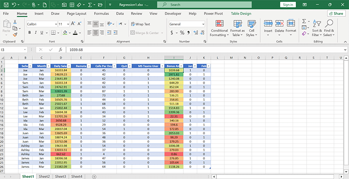
Pic 1
Summery:
The data information of this project is not real. It is taken from an educational collection called “Faradars” and I have made changes in it for educational purposes. The summary of the project is as follows:
A company is considering to check the effect of factors affecting sales and determine the sales target. For this reason, he collected these factors and entered their information in a table. In this table, the names of sales employees are written in the first column. These people provide services remotely or by phone. Some of these people have been fired while working. All employees have been given bonuses by the company manager to motivate them to do more work. The years of experience of the employees are also different.
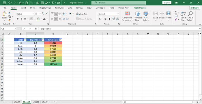
Also, some employees have used “MS Teams user” software to do their work better. The amount of sales is recorded daily for each person, and of course, the total sales of these people are also calculated in a separate table (Pic 2).

Pic 2
The period under review is for the three months of January, February and March. Months of the year are Categorical variable and widen the project review. In order to provide a more detailed analysis, I decided to convert them into dummy variables by including one less number in the number of months and provide the analysis only for the months of January and February.
Since the mathematical model knows only zero and one, wherever the number zero is, it means “No”, and wherever the number one is, it means “Yes”. This method is used to show the presence or absence of some effects of the expected factors.
Investigating the effect of sales factors on the amount of sales requires identifying independent and dependent variables that are analyzed using regression. In this project, the dependent variable is the amount of sales and the independent variables are factors that affect sales.
Dependent variable (Y) = Daily sales, Total sales.
Independent variable (X) = Remote, Calls per Day, Quit, MS Teams User, Bonus Amt, Jan, Feb, Experience.
This project has three parts:
1-The first part: Investigation and influence of independent variables on sales
2-The second part: Investigation and influence of experience on sales
3-The third part: Sales target
Database:
There are 10 columns in this database in sheet 1 and 3 columns in sheet 2:
Seller: The name of the company’s Sellers
Month: Months of activity of sellers
Daily Sales: Daily sales amount in dollars
Remote: Sellers who work remotely
Calls per Day: The number of daily phone calls made by sellers to sell goods
Quit: People who have left their jobs
MS Teams User: It is the name of the software that some sellers have used to sell.
Bonus Amt: The amount of bonus that the manager has planned for the sellers
Jan: Sales in January
Feb: Sales in February
Experience: Number of years and months of work experience
Total Sales: The total sales of each seller in the two months of January and February
Questions & Goals:
1-What is the effect of sales factors as independent variables on daily sales as a dependent variable?
2-Model Fit Summary
3-ANOVA Summary
4-Coefficient Interpretation
5-What are the variables statistically significant?
6-How is the model forecasting?
7-Simplified Model Based on Strong Predictors
8-How does “Experience” predict the target variable?
9-If the seller has 7 years of sales experience, can you predict his/her total sales?
10-How can you determine the sales target based on 7 years of experience?
Steps:
I created two regression models in sheets 3 and 4.
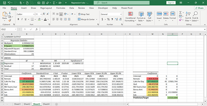
Model 1 (sheets 3): I considered daily sales as the dependent variable and put the factors affecting sales as independent variables. The independent variables at this step were:
Remote, Calls per Day, Quit, MS Teams User, Bonus Amt, Jan, Feb
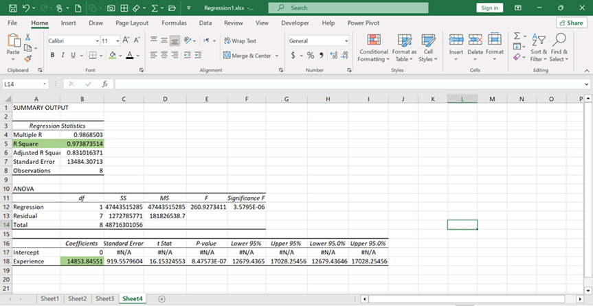
Model 2 (sheets 4): I focused on experience as an independent variable because it seems to be an important factor in sales. And I considered the total sales of each seller as the dependent variable.
Conditional Formatting: Using this tool, the factors that have a greater impact on sales are displayed in green and the factors that have less impact on sales are displayed in red.

Pic 3
Analysis:
-What is the effect of sales factors as independent variables on daily sales as a dependent variable?
Result of Model 1 Evaluations:
R-Square =99%: This is an excellent result. If R-Square be greater than 0.7, it is considered a good result. It means that independent variables or effective factors in sales can explain up to 99% of the dependent variable or sales.
F Significance = 2.26: If the value of the F Significance test is above 5%, the coefficient is not zero. If the coefficient be zero, the independent variable will be zero. This result shows us that there is a linear relationship between our variables.
Standard Error = 789.22: This means that the predicted average is $789.22 away from the actual value. If the sample size increases, the average will be closer to the true value.
Intercept = 0: I considered the Width from origin or fixed value to be zero by default.
P-Value = (0.15, 2.17, 0.95, 0.57, 0.29, 0.628, and 0.621): If it is less than 5%, the coefficient is significant. When F Significance and P-Value are equal, there is only one independent variable. This model shows that the probability of these results is not zero.
Result of Model 2 Evaluations:
R-Square = 97%: This is an excellent result. If R-Square be greater than 0.7, it is considered a good result. It means that independent variables or effective factors in sales can explain up to 97% of the dependent variable or sales.
F Significance = 3.57: If the value of the F Significance test is above 5%, the coefficient is not zero. If the coefficient be zero, the independent variable will be zero. This result shows us that there is a linear relationship between our variables.
Standard Error = 13484.30: This means that the predicted average is $ 13484.30 away from the actual value. If the sample size increases, the average will be closer to the true value.
Intercept = 0: I considered the Width from origin or fixed value to be zero by default.
P-Value = 8.47: If it is less than 5%, the coefficient is significant. When F Significance and P-Value are equal, there is only one independent variable. This model shows that the probability of these results is not zero.
Regression Formulas: Y =ax + b
I use the following formula to determine the amount of sales based on the years of activity:
Sales amount = (X Variable * Sales experience) + Intercept.
In other words, for every one year of sales activity, X Variable amount is added to the sales amount.
-Model Fit Summary
R Square = 0.9988 (99.88%)
This is an extremely high R² value, indicating that 99.88% of the variation in the dependent variable is explained by the model.
Adjusted R Square = 0.9396 (93.96%)
Adjusted R² corrects for the number of predictors.
Even after adjustment, the value remains very high, meaning the model fits extremely well.
Standard Error = 789
This represents the average distance between actual and predicted values.
Given the high R², the standard error is relatively small.
Observations = 24
The model is built on 24 data points acceptable but still a small dataset.
Results should be interpreted carefully due to limited sample size.
-ANOVA Summary
F-statistic ≈ 2029.89
A very large F value shows the regression model is highly statistically significant.
Significance F = 2.26 × 10⁻²²
This is far below 0.05, meaning:
- The overall regression model is statistically significant.
- At least one predictor meaningfully explains the outcome.
-Coefficient Interpretation
Below is an interpretation of each variable using Coefficient + p-value + 95% CI.
Intercept
Coefficient = 0
This is likely due to data scaling or removal of intercept intentionally.
Remote (Coefficient = –454.45, p = 0.1558)
Negative effect: remote workers reduce the predicted target by ~454.
Not statistically significant (p > 0.05).
CI includes zero → uncertainty is high.
Calls Per Day (Coefficient = 377.82, p = 0.0002)
Highly significant positive predictor
Interpretation:
Each additional call increases the target by ≈ 378 units.
Strongest and most significant predictor in the model.
Quit (Coefficient = –38.47, p = 0.515)
Small negative effect.
Not significant (p > 0.05).
CI crosses zero.
MS Teams User (Coefficient = 240.38, p = 0.5716)
Positive effect but not significant.
CI crosses zero.
Bonus Amount (Coefficient = –0.246, p = 0.2375)
Very small and insignificant impact.
Essentially no real measurable effect.
January Dummy (Jan) (Coefficient = 213.90, p = 0.6287)
Positive effect but not significant.
February Dummy (Feb) (Coefficient = 213.46, p = 0.6216)
Also positive but not significant.
-What are the variables statistically significant?
Only one variable is statistically significant:
Calls Per Day
This is the primary driver of the model.
Variables with weak or uncertain effects:
Remote, Quit, MS Teams User, Bonus Amount, Jan, Feb.
All have p > 0.05 → not statistically significant.
Model Strength:
Despite most predictors being insignificant individually, the model overall has a very high R² because Calls per Day is extremely strong. Some predictors may be correlated with each other (multicollinearity).
-How is the model forecasting?
Prediction:
The model calculates a predicted/target value of:
Predicted Value = 17,215.644
This is based on plugging specific variable inputs into the coefficients table.
Final Interpretation
This regression model demonstrates:
Excellent overall fit
One extremely strong predictor (Calls Per Day)
Mostly insignificant secondary predictors
High R² but possible overfitting due to small sample size (24 observations)
-Simplified Model Based on Strong Predictors
Variables with the strongest and most reliable predictive power:
1-Calls Per Day:
Coefficient: +377.8
Interpretation: Higher call volume strongly increases the target variable.
Importance: Very large effect size → one of the main predictors.
2-MS Teams User:
Coefficient: +240.38
Interpretation: Being an MS Teams user is associated with a significant positive increase.
Strong, stable relationship.
Jan and Feb (Seasonality variables):
Coefficients: +213.9 each
Interpretation: Outcomes are consistently higher in January and February.
Importance: These appear to be important seasonal patterns.
Variables to Remove (Weak or Unreliable Predictors)
Remote:
Coefficient is large and negative
But p-value is NOT significant
Confidence interval crosses zero
Not a reliable predictor.
Quit:
Very weak coefficient
Not significant
Offers no predictive value.
Bonus Amt:
Very small coefficient
Not significant
No real contribution.
-How does “Experience” predict the target variable?

Pic 4
Regression Analysis Interpretation:
The regression model shown in the image evaluates how Experience predicts the target variable.
1-Model Fit (Regression Statistics)
Multiple R = 0.9868
This indicates a very strong linear correlation between Experience and the target variable.
R Square = 0.9739 (97.39%)
This means:
Experience explains 97.39% of the variation in the dependent variable.
This is an extremely high R² for a single-predictor model, showing excellent fit.
Adjusted R Square = 0.8310
Adjusted R² penalizes for small sample size (only 8 observations), so the drop is expected.
Still, 0.83 is a strong value.
Standard Error = 13,484
This is the average distance between actual and predicted values.
Given the scale of the coefficient (≈ 14,800), the standard error seems reasonable.
Observations = 8
This is a very small dataset, so results should be interpreted with caution.
Small sample = potential instability in estimates.
2- ANOVA Table
F-statistic = 260.93
A very high F value.
Significance F = 3.57 × 10⁻⁶
This is far below 0.05.
- The regression model is statistically significant.
- Experience is a meaningful predictor of the outcome.
3-Coefficients Interpretation
Intercept
Coefficient = 0
This indicates the intercept was intentionally removed or set to zero.
Experience:
Coefficient: 14,853.85
Standard Error: 919.56
t-stat: 16.15
p-value: 8.47 × 10⁻⁷
95% Confidence Interval:
Lower: 12,679.43
Upper: 17,028.25
Interpretation:
For every 1-unit increase in Experience, the target variable increases by approximately 14,854 units.
This effect is:
- Large
- Positive
- Highly statistically significant (p < 0.000001)
- Confidence interval does NOT cross zero → reliable predictor
4-Overall Interpretation and Insights
Excellent model fit
Experience is explaining nearly all variation in the target.
Experience is a very strong predictor
The effect is large and statistically valid.
Model is statistically significant
The F-test confirms the regression is reliable.
Small sample size (n = 8)
Results should be interpreted cautiously.
With such a small dataset, the model may:
Fit too perfectly
Exaggerate effect size
Be sensitive to outliers
If possible, increasing the dataset size would improve reliability.
5. Final Summary
Experience strongly predicts the target variable.
The relationship is positive, large, and highly significant.
The model explains 97% of variance, which is exceptionally high.
But the dataset is extremely small → interpret with caution.
-If the seller has 7 years of sales experience, can you predict his/her total sales?
Coefficient (β₁) = 14,853.85
Intercept (β₀) = 0
Experience (X) = 7 years
Regression equation:
Sales = 𝛽 0 + 𝛽 1 × 𝑋
Substitute the values:
Sales = 0 + 14,853.85 × 7
Calculation:
14,853.85 × 7 = 103,976.95
Predicted Total Sales = 103,976.95
–How can you determine the sales target based on 7 years of experience?
Sales Target=(Predicted Sales)+(Growth Goal)−(Risk Adjustment)
Predicted = $103,976.95
Growth goal = e.g., 10%
Risk adjustment = e.g., 5%
Target = 103,977 × 1.10 × 0.95 ≈ 108,000
Key points:
- The model is built on 24 data points acceptable but still a small dataset.
- Results should be interpreted carefully due to limited sample size.
- The overall regression model is statistically significant.
- At least one predictor meaningfully explains the outcome.
- The highest impact on factors affecting sales is related to “calls per day” with a factor of 377.81 and the lowest impact is related to “remote” work with a factor of -454.45.
- The highest value of standard error in factors affecting sales is related to “quit” and is equal to 744.83 and the lowest value is related to “bonus” and is equal to 0.299.
- Remote: remote workers reduce the predicted target by ~454.
- Calls Per Day: Highly significant positive predictor
- Quit: Strongest and most significant predictor in the model. Small negative effect.
- MS Teams User: Positive effect but not significant.
- Bonus Amount: Very small and insignificant impact. Essentially no real measurable effect.
- January Dummy (Jan): Positive effect but not significant.
- February Dummy (Feb): Also, positive but not significant.
- Only one variable is statistically significant:
- Calls Per Day, this is the primary driver of the model.
- The model calculates a predicted/target value of: Predicted Value = 17,215.644
- This regression model demonstrates: Excellent overall fit, one extremely strong predictor (Calls Per Day), mostly insignificant secondary predictors, high R² but possible overfitting due to small sample size (24 observations)
- Experience strongly predicts the target variable.
- The relationship is positive, large, and highly significant.
- The model explains 97% of variance, which is exceptionally high.
- But the dataset is extremely small → interpret with caution.
- For every 1-unit increase in Experience, the target variable increases by approximately 14,854 units.
- This effect is: Large, Positive, highly statistically significant (p < 0.000001), Confidence interval does NOT cross zero → reliable predictor
- Results should be interpreted cautiously.
- With such a small dataset, the model may: Fit too perfectly, exaggerate effect size, Be sensitive to outliers
- If the seller has 7 years of sales experience → Predicted Total Sales = 103,976.95
- The sales target based on 7 years of experience → Target = 103,977 × 1.10 × 0.95 ≈ 108,000.
Results & Recommendations:
- If possible, increasing the dataset size would improve reliability.
Recommended Simplified Model:
A clean model using only strong predictors:
Target = 𝛽 0 + 377.8(Calls Per Day) + 240.38(MS Teams User) + 213.9 (January) + 213.46(February)
Target=β 0 + 377.8(Calls Per Day)+240.38(MS Teams User)+213.9(January)+213.46(February)
This model is:
- More stable
- Easier to interpret
- Less prone to overfitting
- Focused on variables with real predictive power
Suggestions to Improve the Regression Model:
1-Increase the Sample Size
This model is built on only 8 observations, which is extremely small for regression.
Why this matters:
High chance of overfitting
Coefficients become unstable
Small sample amplifies random noise
Statistical tests (p-values, confidence intervals) become less reliable
Recommendation:
Try to have at least 30+ observations, ideally 50–100.
2-Check for Outliers
With such a small dataset, one outlier can completely distort the model.
Actions:
Plot a scatter plot of Experience vs Target
Plot residuals to see if any points behave oddly
Remove or investigate extreme values
3-Add More Predictors (if possible)
A single predictor model is simple but may miss important factors.
Examples of useful additional variables:
Education level
Performance metrics
Training hours
Skills rating
Work type (remote/office)
Monthly or seasonal factors
Adding more relevant variables can:
Improve predictive accuracy
Reduce unexplained error
Provide deeper insights
4-Examine Non-Linear Patterns
The relationship between Experience and the target may not be perfectly linear.
Try:
Quadratic term: Experience²
Log transformation: log(Experience)
Polynomial regression
This helps if the effect levels off after a certain point.
Validate the Model
With small datasets, validation is critical.
Techniques:
Leave-one-out cross-validation (LOOCV)
k-fold cross-validation
This shows whether the model generalizes or just fits the noise.
6-Check Assumptions of Linear Regression
Before trusting the model, verify the core assumptions:
- Linearity
- Normality of residuals
- Homoscedasticity (constant variance)
- Independence of errors
7-Consider Adding an Intercept
This model shows:
Intercept = 0
This is likely forced by the Excel regression settings.
Without an intercept, predictions can be biased unless the true relationship genuinely intersects the origin (which is rare). Use a model with an intercept, unless there is mathematical justification to remove it.
8-Standardize Variables (Optional)
If you later add more predictors, standardizing them (z-score) helps:
Compare effect sizes
Reduce multicollinearity
Improve numerical stability
9-Interpret Results Carefully
Given:
Very high R² (97%)
Very small sample
Huge effect size (≈ 15,000 per experience unit)
These values may be inflated because of the limited dataset.
- The obtained coefficients show that those who worked remotely had the least impact on sales and those who had more daily phone calls had the greatest impact on sales. Therefore, it is suggested to remove remote work management from the company’s work contracts or minimize it.
- Bonus are a factor in motivating employees, but contrary to expectations, bonus have had a negative effect on sales, the causes of which must be investigated, whether the amount of the bonus was not appropriate, or the amount of its distribution among people was not fair, or there was another reason.
- The quit factor has had a negative effect on sales, but since it has the highest standard error value, it can be concluded that it is far from the actual value. Since two out of 8 people were fired, it seems that we should increase the number of people in the statistical community in order to get a better result. In this situation, quit was the second negative factor affecting sales and had an impact of -38.47%.
- The use of MS TEAM software has had a positive effect. And it is the second most effective positive factor after the phone call. It is suggested that the management plans to expand its use.
- As a result, the effect of daily phone calls can be considered as the main factor in increasing sales. Considering that the sales in January and February were almost the same, we can consider the hypothetical coefficients and rationalize the targeting.
Action:
In this project, I used simple features and clauses to get my answers:
Features: TABLES, CONDITIONAL FORMATTING, DATA ANALSIS.
Clauses: REGRESSION FORMULAS, F SINGNIFICANCE, STANDARD ERROR, INTERCEPT, P-VALUE, R-SQUER, DEPENDENT VARIABLE, INDEPENDENT VARIABLE.
Link:
Thank you so much for reading my project. I will be happy to receive your feedback and opinion about the project. If this project is useful for you, click on this link:
Link to project repository on GitHub
